Download

1 / 49
490 likes | 553 Views
Learn about the SIFT descriptor for robust image feature matching and detection. Topics include scale invariance, gradient computation, keypoint detection, and properties of SIFT.

E N D
The SIFT descriptor SIFT – Lowe IJCV 2004
Scale Invariant Feature Transform • DoG for scale-space feature detection • Take 16x16 square window around detected feature at appropriate scale • Compute gradient orientation for each pixel • Throw out weak edges (threshold gradient magnitude) • Create histogram of surviving edge orientations: note: each pixel contributes vote proportional to gradient magnitude • Find mode of histogram and rotate patch so that mode is 0 Mode=dominant orientation 2 0 angle histogram Adapted from slide by David Lowe
SIFT descriptor • Create histogram • Divide the 16x16 window into a 4x4 grid of cells (2x2 case shown below) • Compute an orientation histogram for each cell • 16 cells * 8 orientations = 128 dimensional descriptor Adapted from slide by David Lowe
SIFT vector formation • Computed on rotated and scaled version of window according to computed orientation & scale • resample the window
Reduce effect of illumination • 128-dim vector normalized to 1: invariance to contrast changes • Threshold gradient magnitudes to avoid excessive influence of high gradients • after normalization, clamp gradients >0.2 • renormalize
Other tips and tricks • When identifying dominant orientation, if multiple modes, create multiple keypoints • Weigh pixels in center of patch more highly (Gaussian weights) • Trilinear interpolation • a given gradient contributes to 8 bins: 4 in space times 2 in orientation
Linear interpolation into orientation grid A • Blue arrows are centers of orientation bin • Pixel with red orientation contributes to: • Histogram A with weight q • Histogram B with weight p B p q
Bilinear interpolation into spatial grid cells • Blue dots are centers of histograms • Red pixel contributes to: • Histogram A with weight proportional to • Histogram B with weight proportional to • Histogram A with weight proportional to • Histogram A with weight proportional to B A q r p s C D
Properties of SIFT Extraordinarily robust matching technique • Can handle changes in viewpoint • Up to about 60 degree out of plane rotation • Can handle significant changes in illumination • Sometimes even day vs. night (below) • Fast and efficient—can run in real time • Lots of code available: http://people.csail.mit.edu/albert/ladypack/wiki/index.php/Known_implementations_of_SIFT
Summary • Keypoint detection: repeatable and distinctive • Corners, blobs, stable regions • Harris, DoG • Descriptors: invariant and discriminative • spatial histograms of orientation • Next up: using correspondences for reconstruction
The pinhole camera • Let’s abstract out the details
The pinhole camera • We don’t care about the other walls of the box, so let’s remove those
The pinhole camera • Let’s look at a individual points in the world and not worry about what they are.
The pinhole camera Y • Let’s place the origin at the pinhole, with Z axis pointing away from the screen (called camera plane) P = (X,Y,Z) p = (x,y) Z O Z=-1 X
The pinhole camera Y • Let’s remove the wall with the pinhole: all we care about is that all light rays of interest must pass through the pinhole, i.e., the origin P = (X,Y,Z) p = (x,y) Z O Z=-1 X
The pinhole camera Y • Question: Where will we see the “image” of point P on the camera plane? P = (X,Y,Z) p = (x,y) Z O Z=-1 X
The pinhole camera Y P = (X,Y,Z) p = (x,y) Z O Z=-1 X
The pinhole camera Y • Pinhole camera collapses ray OP to point p • Any point on ray OP = • For this point to lie on Z=-1 plane: • Coordinates of point p: p = (x,y) P = (X,Y,Z) Z O Z=-1 X
The projection equation • A point P = (X, Y, Z) in 3D projects to a point p = (x,y) in the image • But pinhole camera’s image is inverted, invert it back!
Another derivation P = (X,Y,Z) Y 1 O y Z p = (x,y,z)
A virtual image plane • A pinhole camera produces an inverted image • Imagine a ”virtual image plane” in the front of the camera P P Y Y 1 O O y y Z 1 Z
Consequence 1: Farther away objects are smaller (X, Y + h, Z) (X, Y, Z) Image of foot: Image of head:
Consequence 2: Parallel lines converge at a point • Point on a line passing through point A with direction D: • Parallel lines have the same direction but pass through different points
Consequence 2: Parallel lines converge at a point • Parallel lines have the same direction but pass through different points
Consequence 2: Parallel lines converge at a point • Need to look at these points as Z goes to infinity • Same as
Consequence 2: Parallel lines converge at a point • Parallel lines have the same direction but pass through different points • Parallel lines converge at the same point • This point of convergence is called the vanishing point • What happens if ?
What about planes? Vanishing line of a plane Take the limit as Z approaches infinity
What about planes? Normal: (NX, NY, NZ) What do parallel planes look like? Vanishing lines Parallel planes converge!
Vanishing line • What happens if NX = NY = 0? • Equation of the plane: Z = c • Vanishing line?
Changing coordinate systems Y Y P = (X,Y,Z) O Z X O’ X Z
Changing coordinate systems Y Y Z X O’ X Z
Changing coordinate systems Y Y Z X O’ X Z
Changing coordinate systems Y Y Z X O’ X Z
Changing coordinate systems Y Y Z X O’ X Z
Changing coordinate systems Y Y Z X O’ X Z
Rotations and translations • How do you represent a rotation? • A point in 3D: (X,Y,Z) • Rotations can be represented as a matrix multiplication • What are the properties of rotation matrices?
Properties of rotation matrices • Rotation does not change the length of vectors
Properties of rotation matrices Reflection Rotation
Rotation matrices • Rotations in 3D have an axis and an angle • Axis: vector that does not change when rotated • Rotation matrix has eigenvector that has eigenvalue 1
Rotation matrices from axis and angle • Rotation matrix for rotation about axis and • First define the following matrix • Interesting fact: this matrix represents cross product
Rotation matrices from axis and angle • Rotation matrix for rotation about axis and • Rodrigues’ formula for rotation matrices
Translations • Can this be written as a matrix multiplication?
Putting everything together • Change coordinate system so that center of the coordinate system is at pinhole and Z axis is along viewing direction • Perspective projection