Introduction to Probability
Introduction to Probability. Experiments Counting Rules Combinations Permutations Assigning Probabilities. These are processes that generate well-defined outcomes. Experiments. Probability is a numerical measure of the likelihood of an event occurring. 0. 1.0. 0.5. Probability:.

Introduction to Probability
E N D
Presentation Transcript
Introduction to Probability • Experiments • Counting Rules • Combinations • Permutations • Assigning Probabilities
These are processes that generate well-defined outcomes Experiments
Probability is a numerical measure of the likelihood of an event occurring 0 1.0 0.5 Probability: The occurrence of the event is just as likely as it is unlikely
Sample Space The sample space for an experiment is the set of all experimental outcomes For a coin toss: Selecting a part for inspection: Rolling a die:
Counting Experimental Outcomes To assign probabilities, we must first count experimental outcomes. We have 3 useful counting rules for multiple-step experiments. For example, what is the number of possible outcomes if we roll the die 4 times? • Counting rule for multi-step experiments • Counting rule for combinations • Counting rule for permutations
Counting Rule for Multi-Step Experiments If an experiment can be described as a sequence of k steps with n1 possible outcomes on the fist step, n2 possible outcomes on the second step, then the total number of experimental outcomes is given by:
Example: Bradley Investments Bradley has invested in two stocks, Markley Oil and Collins Mining. Bradley has determined that the possible outcomes of these investments three months from now are as follows. Investment Gain or Loss in 3 Months (in $000) Collins Mining Markley Oil 8 -2 10 5 0 -20
A Counting Rule for Multiple-Step Experiments Bradley Investments can be viewed as a two-step experiment. It involves two stocks, each with a set of experimental outcomes. Markley Oil: n1 = 4 Collins Mining: n2 = 2 Total Number of Experimental Outcomes: n1n2 = (4)(2) = 8
Tree Diagram Collins Mining (Stage 2) Markley Oil (Stage 1) Experimental Outcomes Gain 8 (10, 8) Gain $18,000 (10, -2) Gain $8,000 Lose 2 Gain 10 (5, 8) Gain $13,000 Gain 8 (5, -2) Gain $3,000 Lose 2 Gain 5 Gain 8 (0, 8) Gain $8,000 Even (0, -2) Lose $2,000 Lose 2 Lose 20 Gain 8 (-20, 8) Lose $12,000 (-20, -2) Lose $22,000 Lose 2
This rule allows us to count the number of experimental outcomes when we select n objects from a (usually larger) set of N objects. Counting Rule for Combinations The number of N objects taken n at a time is where And by definition
Example: Quality Control An inspector randomly selects 2 of 5 parts for inspection. In a group of 5 parts, how many combinations of 2 parts can be selected? Let the parts de designated A, B, C, D, E. Thus we could select: AB AC AD AE BC BD BE CD CE and DE
Ohio Lottery Ohio randomly selects 6 integers from a group of 47 to determine the weekly winner. What are your odds of winning if your purchased one ticket?
Counting Rule for Permutations Sometimes the order of selection matters. This rule allows us to count the number of experimental outcomes when n objects are to be selected from a set of N objects and the order of selection matters.
Example: Quality Control Again An inspector randomly selects 2 of 5 parts for inspection. In a group of 5 parts, how many permutations of 2 parts can be selected? Again let the parts de designated A, B, C, D, E. Thus we could select: AB BA AC CA AD DA AE EA BC CB BD DB BE EB CD DC CE EC DE and ED
Basic Requirements for Assigning Probabilities • Let Ei denote the ith experimental outcome and P(Ei) is its probability of occurring. Then: • The sum of the probabilities for all experimental outcomes must be must equal 1. For n experimental outcomes:
Classical Method This method of assigning probabilities is indicated if each experimental outcome is equally likely
Relative Frequency Method This method is indicated when the data are available to estimate the proportion of the time the experimental outcome will occur if the experiment is repeated a large number of times. What if experimental outcomes are NOT equally likely. Then the Classical method is out. We must assign probabilities on the basis of experimentation or historical data.
Example: Lucas Tool Rental • Relative Frequency Method Lucas Tool Rental would like to assign probabilities to the number of car polishers it rents each day. Office records show the following frequencies of daily rentals for the last 40 days. Number of Polishers Rented Number of Days 0 1 2 3 4 4 6 18 10 2
Relative Frequency Method Each probability assignment is given by dividing the frequency (number of days) by the total frequency (total number of days). Number of Polishers Rented Number of Days Probability 0 1 2 3 4 4 6 18 10 2 40 .10 .15 .45 .25 .05 1.00 4/40
Subjective Method • When economic conditions and a company’s • circumstances change rapidly it might be • inappropriate to assign probabilities based solely on • historical data. • We can use any data available as well as our experience and intuition, but ultimately a probability value should express our degree of belief that the experimental outcome will occur. • The best probability estimates often are obtained by • combining the estimates from the classical or relative • frequency approach with the subjective estimate.
Subjective Method Applying the subjective method, an analyst made the following probability assignments. Exper. Outcome Net Gain or Loss Probability (10, 8) (10, -2) (5, 8) (5, -2) (0, 8) (0, -2) (-20, 8) (-20, -2) $18,000 Gain $8,000 Gain $13,000 Gain $3,000 Gain $8,000 Gain $2,000 Loss $12,000 Loss $22,000 Loss .20 .08 .16 .26 .10 .12 .02 .06