DNS of Surface Textures to Control the Growth of Turbulent Spots

1. DNS of Surface Textures to Control the Growth of Turbulent Spots James Strand and David Goldstein The University of Texas at Austin Department of Aerospace Engineering Sponsored by AFOSR through grant FA 9550-08-1-0453

2. Objectives • There are two primary objectives for the current work: • Examine the structure and properties of large, mature spots at higher values of Rex than in our past work. • Determine whether surface textures continue to be effective at reducing spanwise spreading even as spots are followed significantly further downstream from the initial perturbation. The University of Texas at Austin – Computational Fluid Physics Laboratory

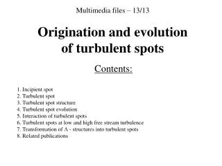
3. Introduction: Turbulent Spots • Boundary layer transition frequently occurs through growth and spreading of turbulent spots. These spots take on an arrowhead shape pointing downstream.1,2 • Spot grows in streamwise, spanwise, and wall-normal directions. 1 Henningson, D., Spalart, P. & Kim, J., 1987 ``Numerical simulations of turbulent spots in plane Poiseuille and boundary layer flow.”Phys. Fluids30 (10) October. 2I. Wygnanski, J. H. Haritonidis, and R. E. Kaplan, J. Fluid Mech. 92, 505 (1979) The University of Texas at Austin – Computational Fluid Physics Laboratory

4. Turbulent Spots – Flow Visualization ReX = 100,000 ReX = 200,000 Visualization of a turbulent spot using smoke in air at different Reynolds numbers.3 ReX = 400,000 3 R. E. Falco from An Album of Fluid Motion, by Milton Van Dyke The University of Texas at Austin – Computational Fluid Physics Laboratory

5. Introduction: Delaying Transition • Drag reduction is a primary means for achieving gains in aircraft fuel efficiency. • Viscous drag is significantly greater for a turbulent boundary layer than for a smooth, laminar boundary layer. • If spanwise spreading of turbulent spots could be constrained, transition might be delayed until further downstream, resulting in lower viscous drag. The University of Texas at Austin – Computational Fluid Physics Laboratory

6. Numerical Method • Spectral-DNS method initially developed by Kim et al.4 • for turbulent channel flow. • Incompressible flow, periodic domain and grid clustering in the direction normal to the wall. • Surface textures defined with an immersed boundary method. • Buffer zone is used to generate the inlet Blasius profile. • Suction wall forces vertical velocity from Blasius solution to allow for correct boundary layer growth downstream. • Initial perturbation which triggers the spot is a small solid body which appears briefly and then is removed. 4J. Kim, P. Moin, and R. Moser, “Turbulence Statistics in Fully Developed Channel Flow at Low Reynolds Number,” J. Fluid Mechanics, Vol. 177, 1987, pp. 133-166. The University of Texas at Austin – Computational Fluid Physics Laboratory

7. Introduction: Surface Textures • Correctly sized riblets reduce turbulent viscous drag ~5-10%.5 • Our past work has shown that surface textures can decrease the spanwise spreading of turbulent spots. • If surface textures can constrain spanwise spreading of spots, turbulent transition might be delayed, leading to significant drag reduction. • Two textures examined: • Triangular riblets • Streamwise fins • The textures are solid, no-slip surfaces. They force all three components of velocity to zero, with the same immersed boundary technique used to create the flat plate. • Relevant parameters for both textures are height, h, and spacing, s. s s h h 5 Bruse, M., Bechert, D. W., van der Hoeven, J. G. Th., Hage, W. and Hoppe, G., “Experiments with Conventional and with Novel Adjustable Drag-Reducting Surfaces”, from Near-Wall Turbulent Flows, Elsevier Science Publishers B. V., 1993 The University of Texas at Austin – Computational Fluid Physics Laboratory

8. Simulation Domain – Comparison to Past Work • 768×192×768 spectral modes in the streamwise (x), wall-normal (y), and spanwise (z) directions, respectively, for a total of 113,246,208 grid points. • Each of these simulations required 36 days to run on 16 processors (13,824 processor hours or ~1.5 processor years). • Our past work used 16,777,216 grid points (so current domain uses more than six times as many). • The domain is 50% longer in each direction than in past work, so total volume of current domain is more than three times greater. • We are able to follow the fully developed spot for twice as long as before. • Rex ≈ 48000 and Reδ* ≈ 377 at the location of the perturbation. • Rex ≈ 298000 and Reδ* ≈ 939 at the end of the domain. The University of Texas at Austin – Computational Fluid Physics Laboratory

9. Simulation Domain • Total of 144 textures (riblets or fins) in each case. • Crest-to-crest spacing for both texture types is 1.1 δo*. • Riblet height = 1.1 δo* and fin height = 0.8 δo*. • Textures start flush with the plate and ramp up to full height over a short distance. The University of Texas at Austin – Computational Fluid Physics Laboratory

10. Results – Flat Wall Spot Isosurfaces of |ωx| showing spot growth. The arrowhead shape becomes more pronounced as the spot matures. Isosurfaces of λ2 for the spot at time t3 above. Note the overhang region at the front of the spot. The University of Texas at Austin – Computational Fluid Physics Laboratory

11. Results – Hairpins Isosurfaces of λ2 help pick out the coherent vortical structures. In this young spot, the hairpins all appear to be of roughly the same size. Viewer is 40° above the horizontal looking down toward the spot and facing downstream. The University of Texas at Austin – Computational Fluid Physics Laboratory

12. Results – Hairpins Same view as previous slide, now showing a more mature spot. There now appears to be a range of hairpin sizes present in the spot. The University of Texas at Austin – Computational Fluid Physics Laboratory

13. Results – Hairpins Same view as previous slide, now showing a large, well-developed spot. A wide variety of hairpin sizes are present in the spot. The University of Texas at Austin – Computational Fluid Physics Laboratory

14. Results – Comparison to Flow Visualizatoin Visualization of a turbulent spot using smoke in air at Rex ≈ 200000. Flat wall spot at Rex ≈ 200000, shown with isosurfaces of λ2. The University of Texas at Austin – Computational Fluid Physics Laboratory

15. Results – Textures vs. Flat Wall The University of Texas at Austin – Computational Fluid Physics Laboratory

16. Results – Textures vs. Flat Wall Riblets Flat Wall Spots over the flat wall, riblets, and fins, shown at the same time step with isosurfaces of λ2. The riblet and fin spots seem to be elongated compared to the flat wall spot. Fins The University of Texas at Austin – Computational Fluid Physics Laboratory

17. Defining the Spot Mature spot shown with two isosurfaces of |ωx|. Translucent blue isosurface is at a lower value (1/4 of the value for the red isosurface). Note that the leading and trailing edge locations are dramatically different depending on which isosurface is used to define them. The University of Texas at Austin – Computational Fluid Physics Laboratory

18. Defining the Spot – Leading and Trailing Edges X-normal plane of integration An integral of |ωx| is calculated for an X-normal plane at each streamwise location. The University of Texas at Austin – Computational Fluid Physics Laboratory

19. Defining the Spot – Leading and Trailing Edges The University of Texas at Austin – Computational Fluid Physics Laboratory

20. Defining the Spot – Leading and Trailing Edges The University of Texas at Austin – Computational Fluid Physics Laboratory

21. Defining the Spot – Leading and Trailing Edges The University of Texas at Austin – Computational Fluid Physics Laboratory

22. Defining the Spot – Leading and Trailing Edges Trailing Edge Leading Edge The University of Texas at Austin – Computational Fluid Physics Laboratory

23. Wingtip Speed • The streamwise location of the wingtip is calculated using three cutoff values of |ωx| for each side of the spot. The wingtip position is then averaged across the centerline to give one value at each time step. These values are plotted against time and a trendline is fit to the data to determine wingtip speed. The University of Texas at Austin – Computational Fluid Physics Laboratory

24. Wingtip, Trailing, and Leading Edge Speeds • Wingtip speeds are very close to trailing edge speeds. • Speeds for the texture cases are very similar to speeds for the flat wall case. • Flat wall trailing edge speed is greater than commonly quoted value of 0.5 U∞, and flat wall leading edge speed is less than commonly quoted value of 0.9 U∞. This is unsurprising since we have defined the leading and trailing edges in a different way than in most previous work. The University of Texas at Austin – Computational Fluid Physics Laboratory

25. Spot Half-Width and Wingtip Location • Three cutoff values of |ωx| are used to get an average edge location for each side of the spot. • Spot half-width is averaged across the spanwise centerline. • Final spot half-width at any given time is an average of 6 total values. Spanwise Extent of the left side of the spot based on the blue isosurface. Spanwise Extent of the right side of the spot based on the red isosurface. The University of Texas at Austin – Computational Fluid Physics Laboratory

26. Spreading Angle • Even once spot is defined, questions remain. Should a virtual origin be used when calculating the spreading angle? The University of Texas at Austin – Computational Fluid Physics Laboratory

27. Virtual Origin Early Spot Developed Spot The University of Texas at Austin – Computational Fluid Physics Laboratory

28. Average Spreading Rate • Plot of spot half-width vs. streamwise locations has many discontinuities. The University of Texas at Austin – Computational Fluid Physics Laboratory

29. Average Spreading Rate • We use the average spreading rate as an additional, alternative measure. • Average spreading rate is proportional to spreading angle as long as spot wingtip moves downstream at a constant speed. The University of Texas at Austin – Computational Fluid Physics Laboratory

30. Spreading • Textures decrease spot spreading by ~7-8% with by either measure. The University of Texas at Austin – Computational Fluid Physics Laboratory

31. Conclusions and Future Work • Conclusions: • Turbulent spots contain a multitude of hairpin vortical structures, entangled with one another throughout the spot. • More mature spots have a broader range of hairpin sizes. • Spot wingtips move at a constant speed, and thus average spreading rate is a reasonable alternative to the spreading angle as a measure of texture effectiveness. • Surface textures are able to reduce the spreading of large, mature spots. Textures examined here reduced spreading by ~7-8% compared to the flat wall value. • Future Work: • Even larger domains might be used to follow spots even further downstream. • Ensemble averaging should be used to further solidify the results of this work. • Turned riblets, as described by Chu et al.6 show promise for achieving greater reductions in spot spreading. They will need to be tested for larger domains at higher Reynolds numbers. 6J. Chu, J. Strand, and D. Goldstein, “Investigation of Turbulent Spot Spreading Mechanism,” AIAA-2010-0716, 48th AIAA Aerospace Sciences Meeting, 4-7 January 2010, Orlando, Florida. The University of Texas at Austin – Computational Fluid Physics Laboratory