Basic Concepts of Stochastic Processes

1. Basic Concepts of Stochastic Processes YangQuan Chen, Ph.D., Director, MESA (Mechatronics, Embedded Systems and Automation)Lab MEAM/EECS, School of Engineering, University of California, Merced E: yqchen@ieee.org; or, yangquan.chen@ucmerced.edu T: (209)228-4672; O: SE1-254; Lab: Castle #22 (T: 228-4398) 9/17/2013. Thursday 09:00-11:15, KL217

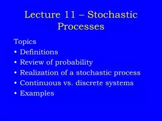
2. Outline • Background on stochastic processes • Gegenbauerprocesses ME280 Fractional Order Mechanics

3. Stochastic Processes [7] Spatial/ensemble Let denote the random outcome of an experiment. To every such outcome suppose a waveform is assigned. The collection of such waveforms form a stochastic process. The set of and the time index t can be continuous or discrete (countably infinite or finite) as well. For fixed (the set of all experimental outcomes), is a specific time function. For fixed t, is a random variable. The ensemble of all such realizations over time represents the stochastic process X(t) or Xt. ME280 Fractional Order Mechanics PILLAI/Cha

4. where is a uniformly distributed random variable in represents a stochastic process. Stochastic processes are everywhere: Brownian motion, stock market fluctuations, various queuing systems all represent stochastic phenomena. (and signals in energy informatics) If X(t) is a stochastic process, then for fixed t, X(t) represents a random variable. Its distribution function is given by Notice that depends on t, since for a different t, we obtain a different random variable. Further represents the first-order probability density function (PDF) of the process X(t). ME280 Fractional Order Mechanics

5. fX(x) x(t) time, t NOTE: PDF only describes the general distribution of the magnitude of the random process, no information on the time or frequency content of the random process ME280 Fractional Order Mechanics

6. For t = t1 and t = t2, X(t) represents two different random variables X1 = X(t1) and X2 = X(t2) respectively with joint distribution given by and represents the second-order density function of the process X(t). Similarly represents the nth order density function of the process X(t). Complete specification of the stochastic process X(t) requires the knowledge of for all and for all n. (an almost impossible task in reality!!). ME280 Fractional Order Mechanics

7. Mean of a Stochastic Process: • represents the mean value of a process X(t). In general, the mean of • a process can depend on the time index t. • Autocorrelation function (ACF) of a process X(t) is defined as • and it represents the interrelationship between the random • variables X1 = X(t1) and X2 = X(t2) generated from the process X(t). • Properties: • 2. (Average instantaneous power) ME280 Fractional Order Mechanics

8. 3. represents a nonnegative definite function, i.e., for any set of constants which follows by noticing that The function represents the autocovariance function of the process X(t). (14-9) ME280 Fractional Order Mechanics

9. Example This gives Similarly ME280 Fractional Order Mechanics

10. Stationary random processes exhibit statistical properties that are invariant to shift in the time index. For example, second-order stationarity implies that the statistical properties of the pairs {X(t1) , X(t2) } and {X(t1+c) , X(t2+c)} are the same for anyc. Similarly first-order stationarity implies that statistical properties of X(ti) and X(ti+c) are the same for any c. In strict terms, the statistical properties are governed by the joint probability density function. Hence a process is nth-order Strict-Sense Stationary (S.S.S)if for anyc, where the left side represents the joint density function Of the random variables and the right side corresponds to the joint density function of the random variables A process X(t) is said to be strict-sense stationary if it is true for all Stationarity ME280 Fractional Order Mechanics

11. For a first-order strict sense stationary process, for any c. In particular c = – t gives i.e., the first-order density of X(t) is independent of t. In that case Similarly, for a second-order strict-sense stationary process we have for any c. For c = – t2 we get ME280 Fractional Order Mechanics

12. So, the second order density function of a strict sense stationary process depends only on the difference of time indices In that case the autocorrelation function is given by i.e., the autocorrelation function of a second order strict-sense stationary process depends only on the difference of the time indices the basic conditions for the first and second order stationarity are usually difficult to verify. In that case, we often resort to a looser definition of stationarity, known as Wide-Sense Stationarity (W.S.S). ME280 Fractional Order Mechanics

13. A process X(t) is said to be Wide-Sense Stationary (W.S.S)if • and • (ii) • i.e., for wide-sense stationary processes, the mean is a constant and • the autocorrelation function depends only on the difference between • the time indices. WSS does not say anything about the nature of • the probability density functions (PDF), and instead deal • with the average behavior of the process. Note: strict-sense • stationarity always implies wide-sense stationarity. However, the • converse is not true in general, the only exception being the • Gaussian process. PILLAI/Cha ME280 Fractional Order Mechanics

14. Averaging and stationarity • Ensemble averaging: properties of the process are obtained by averaging over a collection or ‘ensemble’ of sample records using values at corresponding times • Time averaging: properties are obtained by averaging over a single record in time • Stationality: Ensemble averages do not vary with time • Ergodicity: stationary process in which averages from a single record are the same as those obtained from averaging over the ensemble ME280 Fractional Order Mechanics

15. A deterministic system1 transforms each input waveform into an output waveform by operating only on the time variable t. Thus a set of realizations at the input corresponding to a process X(t) generates a new set of realizations at the output associated with a new process Y(t). Our goal is to study the output process statistics in terms of the Input process statistics and the system function. 1A stochastic system on the other hand operates on both the variables t and Systems with Stochastic Inputs ME280 Fractional Order Mechanics

16. Deterministic Systems Memoryless Systems Systems with Memory Time-Invariant systems Linear systems Time-varying systems Linear-Time Invariant (LTI) systems LTI system ME280 Fractional Order Mechanics

17. Memoryless Systems The output Y(t) in this case depends only on the present value of the input X(t). i.e., Strict-sense stationary input Memoryless system Strict-sense stationary output. Need not be stationary in any sense. Wide-sense stationary input Memoryless system Y(t) stationary,but not Gaussian with X(t) stationary Gaussian with Memoryless system ME280 Fractional Order Mechanics

18. wide-sense stationary process LTI system h(t) wide-sense stationary process. (a) strict-sense stationary process LTI system h(t) strict-sense stationary process (see Text for proof ) (b) Linear system Gaussian process (also stationary) Gaussian process (also stationary) (c) LTI Systems (with memory) ME280 Fractional Order Mechanics

19. White Noise Process W(t) is said to be a white noise process if i.e., E[W(t1) W*(t2)] = 0 unless t1 = t2. W(t) is said to be wide-sense stationary (w.s.s) white noise if E[W(t)] = constant, and If W(t) is also a Gaussian process (white Gaussian process), then all of its samples are independent random variables (why?). For w.s.s. white noise input W(t), we have LTI h(t) White noise W(t) PILLAI/Cha ME280 Fractional Order Mechanics

20. and where Thus the output of a white noise process through an LTI system represents a (colored) noise process. Note: White noise needs not be Gaussian. “White” and “Gaussian” are two different concepts! (14-44) (14-45) (14-46) PILLAI/Cha ME280 Fractional Order Mechanics

21. Input x(t) Output y(t) Linear system Sy(n) Sx(n) A.|H(n)|2 frequency, n Unit: W*sec. Power Spectral Density (PSD): ACF (or autocovariance): W W ME280 Fractional Order Mechanics

22. Periodogram: Approximation of PSD Given an observed sequence X1, …, Xn , define ME280 Fractional Order Mechanics

23. Discrete Time Stochastic Processes A discrete time stochastic process Xn = X(nT) is a sequence of random variables. The mean, autocorrelation and auto-covariance functions of a discrete-time process are gives by and respectively. As before strict sense stationarity and wide-sense stationarity definitions apply here also. For example, X(nT) is wide sense stationary if and ME280 Fractional Order Mechanics

24. Consider an input – output representation where X(n) may be considered as the output of a system {h(n)} driven by the input W(n). Z – transform gives or h(n) W(n) X(n) Auto Regressive Moving Average (ARMA) Processes ME280 Fractional Order Mechanics

25. ARMAX (Auto Regressive Moving Average eXtra input) • Same denominator A(q) is used for both transfer functions • A(q)y(n) represents an auto-regression (AR) • C(q)e(n) represents the moving average of white noise (MA) • B(q)e(n) represents an extra (exogenous) input • In ARMAX model, the noise and input signal are subjected to the same dynamics • This is particularly suitable for a process where dominating disturbance enters the process at the point of input ME280 Fractional Order Mechanics

26. Box-Jenkens ME280 Fractional Order Mechanics

27. Outline • Background on stochastic processes • Gegenbauerprocesses ME280 Fractional Order Mechanics

28. Motivations: Long Memory or LRD Concept of persistency – shot responses short memory long memory DOI 10.1007/s00477-005-0029-y ME280 Fractional Order Mechanics

29. SRD vs LRD • Short-range dependent (SRD) processes are characterized by an autocorrelation function which decays exponentially fast; • Long-range dependence (LRD) processes exhibit a much slower decay of the correlations - their autocorrelation functions typically obey some inverse power law. http://en.wikipedia.org/wiki/Long-range_dependency ME280 Fractional Order Mechanics

30. Mathematically, • A stationary process is said to have long-range correlations if its covariance function C(n) (assume that the process has finite second-order statistics) decays slowly as n→∞, i.e. for 0 < α < 1, where c is a finite, positive constant. • The weakly-stationary time-series X(t) is said to be long range dependent if its spectral density obeys f(λ) ∼ Cf |λ|−βas λ → 0, for some Cf > 0 and some real parameter β ∈ (0, 1). ME280 Fractional Order Mechanics

31. Heavy tailedness and Long tailedness • The distribution of a random variable X with distribution function F is said to have a heavy right tail if • The distribution of a random variable X with distribution function F is said to have a long right tail if for all t > 0, NOTE: long-tailed distributions are heavy-tailed, but the converse is false if you know the situation is bad, it is probably worse than you think. http://en.wikipedia.org/wiki/Heavy-tailed_distribution ME280 Fractional Order Mechanics

32. SRD and LRD models • SRD • AR, ARMA, Markov processes, white noise • LRD • ARFIMA or FARIMA, fractional order models, Gegenbauer model ME280 Fractional Order Mechanics

33. 100+ years of LRD/HT research • Distribution of wealth, income of individuals • City sizes vs. ranks - given the population, what is the city rank? • Graphs of gene regulatory & protein-protein networks are scale free • Long neuron inter-spike intervals in depressed mice • Internet and WWW - scale free network (graph): fault tolerant, hubs are both the strength and Achilles’ heels • Scene lengths in VBR and MPEG video are heavy-tailed • Computer files, Web documents, frequency of access are heavy-tailed • Stock price fluctuations and company sizes • Inter occurrence of catastrophic events, earthquakes - applications to reinsurance • Frequency of words in natural languages (often called Zipf’s law) Ubiquity of Power Laws, Jankovic, 2007 ME280 Fractional Order Mechanics

34. ARFIMA/FARIMA model Fractional autoregressive integrated moving average (B=z-1) Fractional differencing: ME280 Fractional Order Mechanics

35. ARFIMA ARFIMA(0,d,0): FI(d) ACF: ARFIMA: both long memory and short memory in autocorrelation structure ME280 Fractional Order Mechanics

36. Gegenbauer Polynomial C(α)n(x) • Generating function: • Recurrent relation ME280 Fractional Order Mechanics

37. Gegenbauer Process Xt • ACF structure: • Using Gegenbauer polynomial property ME280 Fractional Order Mechanics

38. Gegenbauer Process Xt • Infinite MA expression • Note: ME280 Fractional Order Mechanics

39. Properties of Gegenbauer Process Xt PSD: Singularity: So when 0<d<1/2, unbounded PSD with persistent cyclic component of frequency ME280 Fractional Order Mechanics

40. GARMA(p,d,q,η) model • Genenbauer (generalized) ARMA model • When η=1, GARMA(p,d,q,η) becomes ARFIMA(p,2d,q)! • GARMA(0,0,d,1) reduces to FI(2d). ME280 Fractional Order Mechanics

41. k-factor Gegenbauer Process • Model: • ACF: complicated! • PSD: Okay format: So better work in spectral domain Gegenbauer frequency: ME280 Fractional Order Mechanics

42. Simulation Illustration 3-factor Gegenbauer process simulated with (d1=0.45, d2=0.35, d3=0.30), (ν1=0.9, ν 2=0.5, ν 3=0.1) and σ2=1. [3] ACF PSD ME280 Fractional Order Mechanics

43. k-factor Gegenbauer ARMA (GARMA) model ME280 Fractional Order Mechanics

44. Parameter Estimation (Sadek and Khotanzad, 2004) ME280 Fractional Order Mechanics

45. ME280 Fractional Order Mechanics