Morgan Ulloa March 20, 2008
370 likes | 578 Views
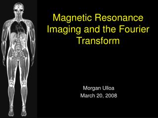
Magnetic Resonance Imaging and the Fourier Transform. Morgan Ulloa March 20, 2008. Outline. The Fourier transform and the inverse Fourier transform Fourier transform example 2-D Fourier transform for 2-D images Magnetic Resonance Imaging (MRI) Basic MRI physics

Morgan Ulloa March 20, 2008
E N D
Presentation Transcript
Magnetic Resonance Imaging and the Fourier Transform Morgan Ulloa March 20, 2008
Outline • The Fourier transform and the inverse Fourier transform • Fourier transform example • 2-D Fourier transform for 2-D images • Magnetic Resonance Imaging (MRI) • Basic MRI physics • K-Space and the inverse Fourier transform • Overview of how an MRI machine works • 3-D MRI
What is the Fourier transform • A component of Fourier Analysis named for French mathematician Joseph Fourier (1768-1830) • The Fourier transform in an operator that inputs a function and outputs a function • Inputs a function in the time-domain and outputs a function in the frequency-domain • the Fourier transforms is used in many different ways • Continuous Fourier transform is used for MRI
What the Fourier transform looks like • Written as an integral: • f(t) is a function in the time-domain • ω=2πf known as the angular frequency • i = square root of -1 (imaginary number) • t is the variable time • The Fourier transform takes a function in the time-domain into the frequency-domain
Inverse transform • Also an integral: • F(ω) is our Fourier transform in the frequency-domain • ω=2πf known as the angular frequency • i is the square root of -1 • t is the variable time • 1/(2 π)is a conversion factor • The inverse Fourier transform takes a function in the frequency-domain back into the time-domain
Example: 1) Define time-domain function 2) Compute our integral: = • Improper integral = = Note: Has a real part and an imaginary part
from the definition of the integral of products of trigonometric functions = simplifying the fractions = 3) Understanding what this means - searching for a specific frequency (ω)
Begin with a 2-D array of data:t’byt’’ Since this data is two dimensional we say that the data is in the spatial domain The 2-D Fourier transform
1st Fourier Transform First Fourier transform in one direction: t’
2nd Fourier Transform Finally in the t’’ direction The spike corresponds to the intensity and location of the frequency within the 2-D frequency domain
What is MRI? • Originally called nuclear magnetic resonance (NMR) but now it is called MRI in the medical field because of negative associations with the word nuclear • Thus, on the atomic level MRI utilizes properties of the nucleus, specifically the protons • It takes tomographic images of structures inside the human body similar to an x-ray machine • Unlike the x-ray this imaging technique is non-ionizing
Tomography • Tomography: slice selection, with insignificant thickness, of a 3-D object
Spin and spin states • Certain atoms have protons that create tiny magnetic fields in one of two directions: this is called spin • some common and important types of atoms with this property are 1H, 13C, 19F, 31P • Hydrogen protons are used for MRI in the human body • Usually the spins of protons in a compound are oriented randomly but if they are exposed to a magnetic field they either align themselves with it, called parallel alignment, or against it, called antiparallelalignment. • The parallel and antiparallel alignments are called spin states • The energy difference between the spin states lies within the radio frequency spectrum
Resonance • When a magnetic field is applied the protons oscillate between their two spin states: between antiparallel and parallel alignment • A radio frequency is applied by the MRI machine and varied until it matches the frequency of the oscillation: this is called resonance • Whilst in this state of resonance the protons will absorb and release energy • This is then measured by a radio frequency receiver on the MRI machine • The energy difference of the two spin states depends on the response of protons to the magnetic field in which it lies and, since the magnetic field is affected by the electrons of nearby atoms, each MRI scan produces a spectrum that is unique to the compounds present in the tomographic slice
Radio Frequency Spectrum • Spectrum:the distribution of energy emitted by a radiant source
x-axis called the phase-encoding axis y-axis called the frequency encoding axis Axes of a 2-D slice
A region of spin is simply a location within the 2-D slice plane where protons are expressing their unique characteristic: spin For the purposes of explaining the 2-D Fourier transform we will use 2 regions of spin with similar material compositions but different locations: labeled 1 and 2 Regions of spin
Imagining these regions of spin • These regions of spin can be depicted visually by vectors (magnetization vectors) rotating around the origin at a frequency corresponding to their rates of oscillation
x-axis: Phase Encoding • Magnetic field gradient is applied to the slice along the x-axis to both regions of spin • The radio frequency bursts are applied and both regions of spin resonate at different frequencies because they have different positions • when the gradient is turned off they will have a different phase angle,φ • Phase angle: the angle between the reference axis (y) and the magnetization vectors
y-axis: Frequency encoding • The magnetic field gradient is then applied along the y-axis • This results in the two spin vectors rotating at unique frequencies about the origin • Thus each region of spin now has a unique rotational frequency and a unique phase angle
Using the Fourier transform with this data • Mapping these rotations about the origin as functions of time we get two unique time-domain signals each with a unique phase and rotational frequency and we can create a 2-D array of data with our rows and columns • To these we can apply the Fourier transform as we did before in the t’ and t’’ directions but this time in the frequency encoding direction and the phase encoding direction • therefore our data is in the spatial domain, not the time domain as with 1-D Fourier transform • This process identifies the the position and the intensity of the spin within the 2-D slice plane
We have our two unique signals plotted as a 2-D array of data A visual of how this works…
… • First Fourier transform in the frequency encoding direction
Then Fourier transform in the phase encoding direction The spikes indicate frequency intensity and location of our regions of spin …
What is the K-space? • A matrix known as a temporary image space which holds the spatial frequency data from a 2-D Fourier transform • The number of entries in each row and column correspond to the number of regions of spin within the slice plane and their location • Each matrix entry is given a pixel intensity and thus each entry contains both frequency and spatial data • These entries form a grayscale image • Whiter entries correspond to high intensity signals • Darker entries correspond to low intensity signals
The k-space for our two regions of spin is the following matrix which clearly demonstrates the position and intensity (here the difference in color) of each region K-space for the two regions of spin
From the K-space to a recognizable image • Inverse transforming the K-space yields a new grayscale image that corresponds to the physical slice plane, thus creating an accurate image representation of the slice in vivo
MRI imaging process • A slice is selected from the body • Magnetic Field gradient is applied to the slice in the Phase encoding and Frequency encoding directions • only the protons within the slice to oscillate between their two energy states (spin states) • At the same time radio frequency pulses are applied to the slice with a bandwidth capable of exciting all resonances simultaneously • The emitted energy is measured by a radio frequency receiver and converted into a spectrum in the time-domain in the x-direction and y-direction thereby creating a 2-D array of data in the spatial domain
…MRI process continued • The two time-domain functions of the spatial-domain is then Fourier transformed into a 2-D frequency-domain function with information about the position and frequency intensity of the spin regions • This data is entered into the K-space and then inverse Fourier transformed creating a corresponding accurate image of the physical slice
References: • Campbell, Iain D., and Raymond A. Dwek. Biological Spectroscopy. Menlo Park, Ca: Benjamin/Cummings Company, 1984. • Gadian, David G. Nuclear Magnetic Resonance and Its Applications to Living Systems. New York: Oxford UP, 1982. • Hornak, Joseph P. "The Basics of MRI." 1996. Rochester Institute of Technology. 30 Sept. 2007 <http://www.cis.rit.edu/htbooks/mri/>. • Hsu, Hwei P. Applied Fourier Analysis. Orlando: Harcourt Brace Jovanovich, 1984. • Knowles, P. F., D. Marsh, and H.W.E. Rattle. Magnetic Resonance of Biomolecules. John Wiley & Sons, 1976. • Mansfield, P., and P. G. Morris. NMR Imaging in Biomedicine. New York: Academic P, 1982. • Swartz, Harold M., James R. Bolton, and Donald C. Borg. Biological Applications of Electron Spin Resonance. John Wiley & Sons, 1972.
Many thanks toProfessor Ron Buckmire & the Occidental Mathematics Department