Download
1 / 1
30 likes | 234 Views
*Contact: toni.galvin@unh.edu.

E N D
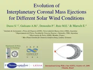
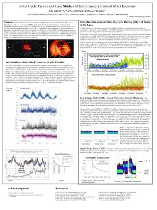
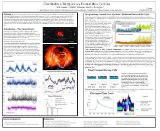
*Contact: toni.galvin@unh.edu Abstract We contrast the solar wind characteristics for interplanetary coronal mass ejections (ICME) cases at different phases of the solar cycle using STEREO observations. The Plasma and Suprathermal Ion Composition (PLASTIC) instruments on the twin spacecraft STEREO A (STA) and STEREO B (STB) were commissioned in January 2007 and have been operating continuously (orbit, Fig. 1). The mission to date encompasses the decline into the solar minimum of December 2008 and predicted maximum of cycle 24 (Fig. 2). The PLASTIC investigation measures the solar wind protons, alphas, and selected minor ions. This past solar minimum was characterized by weak transients. In contrast the rising solar cycle included extremely fast ICMEs, with one such ICME observed in situ by STEREO A exceeding 1500 km/s at 1 AU. We will compare specific cases of slow and fast ICME solar wind, as observed in situ by STEREO, to general solar wind parameters, particularly for iron ions. • Interplanetary Coronal Mass Ejections – Different Phases of the Cycle • Of particular interest to the mission objectives of the STEREO mission are the identification of the passage of interplanetary coronal mass ejections (ICMEs). For ICME identification, PLASTIC provides the proton and alpha bulk parameters and ionic charge states of selected minor species, such as iron. • Low Charge State ICMEs – Small Transients. Using STEREO and near Earth assets, this recent solar minimum revealed a number of small transients (ST), as first reported by Kilpua et al. (2009, 2012), and later by Yu et al. (2013). In some cases, the origins have been tracked. Foullon et al. (2011) detected a detached plasmoid in the heliospheric plasma sheet (HPS) associated with the heliospheric current sheet (HCS). Rouillard et al. (2011) linked plasmoid release observed remotely to in-situ observations. • Charles Farrugia and Wenyuan Yu have used STEREO A, STEREO B, and Wind to identify small transients during the recent solar minimum period (2007-2009). Their selection criteria included: (1) Duration less than 12 hrs, (2) Low Tkin and/or low beta, (3) Enhanced magnetic field strength relative to 3 year average, and one or more of the following: (4) Decreased B variability, (5) Large, coherent rotation of the field vector, (6) Low Alfven Mach number, and/or (7) Te/Tp higher than 3 year average. They found 126 samples: Average duration was 4.3 hours, with 75% less than 6 hours; 81% of which were in the slow solar wind (Vp < 450 km/s). Many start or end with sharp field discontinuities. Year 2009 was the bumper crop. They found one main difference from longer duration ICMEs during the same interval was that the Tkinetic was not “cold” compared to expectations. (ICMEs often have low Tkin’s). In addition, as shown here (Fig 7), the composition was indistinguishable from the ambient solar wind. • High Charge State ICMEs. The highest Fe<Q> observed to date on STA is during the July 2012 magnetic cloud event. This event is considered a “Carrington Class” due to its high speeds and magnetic fields (Russell et al., 2013). Figure 6 Shown in Fig. 6 are the daily average helium relative abundance and iron ionic charge state Fe<Q>, derived from hourly accumulations, observed by STA PLASTIC from commissioning through 2013. As expected, the occurrence frequency of higher Fe<Q> and He/H events is increasing with the approach to solar maximum. These instances are sporadic, lasting several minutes to days, and have been identified as a robust signature of an ICME passage. However, although high ionic charge states are a reliable indicator of an ICME (e.g., Reinard, 2008), not all ICMEs exhibit extreme composition. The ICMEs observed during this past solar minimum were typically characterized by very modest Fe charge states, as reported by Galvin et al. (2009, 2011). Jian et al. (2011) report that the ICMEs in the recent solar minimum were smaller, slower and weaker than those observed during the 1996 minimum. Introduction – The Current Cycle Solar wind data near Earth are routinely available from the mid 1960’s onwards thanks to NASA’s OMNI-2 data compilation (King and Papitashvilli), providing a tremendous resource for both event-oriented and long-term studies. With the STEREO data set, we also acquire, for the first time, continuous longitudinal data at 1 AU (Fig. 1,4). General solar wind trends for the current solar cycle indicate that there are differences in this cycle from earlier cycles. Coronal holes, dominant during solar minimum, are associated with higher speeds and higher kinetic temperatures, creating a modest correlation of these parameters with the minimum cycle phase. Note however the significant low speeds (Fig 3-blue oval, Fig. 4-5) and kinetic temperatures (Fig. 3-blue oval) observed in the 2009 solar wind during the sustained recent solar minimum. A reduced mass flux has also been observed (Fig. 3), which has implications for magnetospheric and heliospheric boundaries (McComas et al., 2013). With STEREO, we confirm that these trends are seen at all longitudes when long term averages are used (e.g., Fig. 4, 27-day running averages). Figure 1 Case Studies of Interplanetary Coronal Mass Ejections Figure 2 STEREO Figure 3 Omni-2 Figure 4 Figure 7. Composition for three small transient events, identified by Yu et al (2013). Shown from top to bottom for each day of an event period: the iron charge state distribution (top), average and peak Fe charge state (middle), and the iron solar wind speed (bottom). The start and stop times of the transient interval are shown below their respective figure. All 45 events for STEREO A used in Yu et al (2013) were analyzed. They all looked like this. A.B. Galvin*1,2, K.D.C. Simunac1 and C.J. Farrugia1,2 1.Space Science Center, Institute for the Study of Earth, Oceans and Space, 2. Department of Physics, University of New Hampshire Speed Minimum late 2009 Figure 8 STEREO A PLASTIC Transient Solar Wind Charge States (Note: Fe Q ≥ 22) Figure 5 Ambient Solar Wind Charge States • Acknowledgments • NASA STEREO Grant NNX13AP52G at UNH • J. H. King and N. Papitashvilli at NASA GSFC and CDAWeb for the ONMI data. • References • Foullon, C., et al, doi 10.1088/0004-637X/737/1/16, 2011. Galvin, A.B., et al., Ann. Geophys., 27, 3909-3922, 2009.Galvin, A.B., doi 10.1007/978-90-481-9787-3_11, 2011. • Jian, L.K., C.T. Russell, and J.G. Luhmann, Solar Phys., 274:321-344, 2011. Kilpua, EKJ, et al, doi 10.1007/s11207-009-9366-1, 2009. Kilpua, EKJ, et al, doi: 10.1007/s11207-012-9957-0, 2012. • McComas, D., et al., doi 10.1088/0004-637X/779/1/2, 2013. Rouillard, AP., et al., doi 10.1088/0004-637X/734/1/7, 2011. Reinard, A.A., Astrophysical Journal, 682:1289-1305, 2008. • Russell, CT., et al., doi 10.1088/0004-637X/770/1/38, 2013. Yu, W., et al., doi 10.1002/2013JA019115, 2013.