Download
1 / 24
240 likes | 258 Views
Explore the concept of Open Boundary Conditions (BCs) in quantum physics, allowing the addition and removal of charge in systems. Learn about changing viewpoints and system responses to external stimuli. Discover the significance of contacts in altering charge dynamics and broadening energy states.

E N D
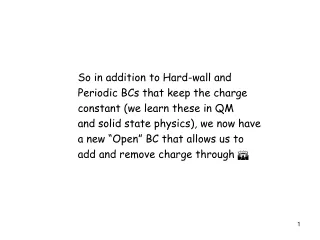
So in addition to Hard-wall and Periodic BCs that keep the charge constant (we learn these in QM and solid state physics), we now have a new “Open” BC that allows us to add and remove charge through S
Hard Wall Boundary Conditions x 0 -t e -t -t e -t H = -t e -t Time 0 Hard Wall U Hard Wall SetH = 0 at ends
Periodic Boundary Conditions x -t -t e -t -t e -t H = -t e -t Time -t Wrap around U SetH = -t at ends
Open Boundary Conditions x -teika 0 0 0 0 0 0 S1 = S2 = 0 0 -t e -t -t e -t H = -t e -t Time Time -teika with E = e-2tcoska To infinity and beyond U To –infinity and beyond Need a S which does this
But notice that in addition to different BCs, we are also changing our viewpoint, since we are talking of an open system now to which we can add or remove charge
Altering viewpoint x Time Note how we can’t talk of eigensolutions of an open system, since all energies are allowed Instead we talk of response (G) of the device to electrons impingent at all energies This entails a major change of viewpoint. Instead of looking for modes of the quantum strings, we are looking for the response of the string to tuning forks (incident electrons) at different excitation frequencies (energies)
x w Time So far We now see how contacts add and remove charge and impose a finite lifetime They also impose broadening Eigenmodes Resonant modes
A B C D EI-H -t -t+ (E+ih)I – HR (A-BD-1C)-1 G∞ = Another derivation G∞ = [(E+ih)I-H∞]-1 for entire system -1 -1 = = From simple algebra
S Another derivation Thus, we get the device block of G: [(EI-H-tgRt+]-1 G = where gR = [(E+ih)I-HR]-1 Advantage: often t connects only 1st element of contact Green’s function, g with device H ie, S = tgt+, where the surface Green’s function g satisfies a recursive relation
g1 g -b a -b+ -b a -b+ gR = -b a -b+ Contact Green’s Fn Recursive Equation g = (a – bgb+)-1 Equation g = (a – bg1b+)-1 Device -1 If a = E-2t0, • = -t0 and E = Ec+2t0(1-coska) Then this gives g = -1/t0.eika S = tgt+ = t02g = -t0.eika
Sum Rule 1 0 0 1 A(E)dE/2p = = I For our 2x2 case Since I matrix is basis-invariant, true in non-eigenspace too Thus, integrating states over energy gives 1 at each point (SUM RULE for LDOS at every individual atomic site)
In 1-D g satisfies recursive equation g = (a – bgb+)-1 (a,b are onsite and hopping terms of EI-H) To summarize iħdy/dt –Hy – Sy = S Self Energy S = tgt+ where g is contact surface Green’s fn, t couples it to device AntiHermitiain part gives broadening G = i(S-S+) Turns out Hermitian and anti-Hermitian parts are related !
Quick and dirty estimates If we don’t want to do all that algebra, can simply assume G ≈ ħv/a (true in 1-D, but ‘a’ hard to define in general 3-D) Real part of S is constrained by G (must be, to retain sum-rule) S = H[G], ie, Hilbert Transform SR(E) = dE’G(E’)/(E-E’) Physicists call this Kramers-Kronig
Quick and dirty estimates Im(S) ~ DOS Im(S) ~ DOS • S = H[G], ie, Hilbert Transform • SR(E) = dE’G(E’)/(E-E’) Physicists call this Kramers-Kronig Re(S) Re(H(G)) E E
More realistic DOS plots Magnet (Fe) UP DOWN s,p d-band Semic (Si) Metal (Gold) Bulk Reconstructed
gate Giving us same two eigenstates out of one atom provided S is energy-dependent Energy-dependent S can capture bonding chemistry Has two energy eigenvalues Could treat one atom as ‘contact’ on another “Self-energy” can capture chemistry
gate Broadening of 1 level by another G = t2 x h/[ (E-e2)2 + (h/2)2] “Self-energy” can capture chemistry So any part of a device can act like a ‘contact’ on the other But it may not be a ‘well-behaved’ contact (ie, reservoir which is unaffected by device dynamics) Depends sensitively on our choice for h
e Broadening of 1 level by many others with almost equal coupling What makes a good contact? Aside from making G ind. of device, we’d also like Gf (inflow) to be unaffected by device This requires contact to stay at equilibrium, which happens if there’s good communication (scattering) among contact levels so energy is redistributed and kept at f (Ch 10) G(E) = deDR(e) x t2 x h/[(E-e)2 + (h/2)2] = 2pt2DR(E) Ind. of h (Fermi’s Golden Rule) ≈ DR(E)t2deh/[(E-e)2 + (h/2)2]
To summarize • We learned how to include open BCs (contact) through source and self-energy which we can calculate given atomic properties (a,b of contacts gives g-1 = (a-bgb+), t of interface gives S = tgt+) • Contact creates finite lifetime for device electrons and turns sharp eigen-states into broadened resonant states • Broadening G and lifetime t = ħ/G have inverse relation mediated by factor of ħ (Uncertainty Principle) • We defined Spectral Function, Local DOS and Sum-rule • An ‘ideal’ contact has many levels that make its broadening G and occupancy f independent of device dynamics
How to get Scatt. pics at start? S = 0 (open bcs) S(1,N) = S(N,1) = -t (periodic bcs) Add self-energy for BCS S1(1,1) = S2(N,N) = -teika (open bcs) -t e -t -t e -t H = -t e -t Initial state j0 = (1/s2p)e-ikxexp[-(x-x0)2/2s2] (Normalized Gaussian packet, with a initial velocity ħk/m) Add pot. U (barrier between x1, x2) How do we solve time-dep. SE given H, U, S and initial condition j0? iħdj/dt = Hj
How to solve time-dep. SE? One approach: Crank-Nicholson algorithm jt+Dt = (I-iHDt/2ħ).(I+iHDt/2ħ)-1jt Convert j into matrix with rows along x, columns along t Convert SE by using finite difference: Hjt = iħdjt/dt ≈ iħ(jt+Dt – jt)/Dt Thus, jt+Dt ≈ (I-iHDt/ħ)jt = Ujt But transformation must be UNITARY to conserve probability |jt|2 over time, ie, must construct U such that UU+ = I
Result Hard wall bcs Periodic bcs Open bcs
% Time-dependent SE showing scattering of particle from potential, % And hard walls clear all Nx=101;x=linspace(0,100,Nx);dx=x(2)-x(1); % real space grid sig=8;x0=20;k=1; % parameters for wavepacket distribution Nb=20;k=2*pi/(Nb+1); %for resonance in RTD psi=exp(-i*k*x).*1/(sig*sqrt(2*pi)).*exp(-(x-x0).^2/(2*sig^2)); H=2*eye(Nx)-diag(ones(1,Nx-1),1)-diag(ones(1,Nx-1),-1); % Create potential %Nd=3;V=blkdiag(zeros(40),eye(Nx-40)); % Step %Nd=30;V=blkdiag(zeros(40),-eye(Nd),zeros(Nx-40-Nd)); % Well Nd=30;V=blkdiag(zeros(40),0.5*eye(Nd),zeros(Nx-40-Nd)); % Barrier %Nb=20;Nw=20;V=blkdiag(zeros(20),eye(Nb),zeros(Nw),eye(Nb),zeros(Nx-20-Nw-2*Nb)); %RTD %V=V+diag(linspace(0,1,Nx));%Field H=H+V; % Boundary condition %sig=zeros(Nx); % Hard wall %s1=-exp(i*k);s2=s1;sig1=zeros(Nx);sig(1,1)=s1;sig(Nx,Nx)=s1; % Open boundary conditions sig=zeros(Nx);sig(1,Nx)=-1;sig(Nx,1)=-1; % Periodic boundary conditions H=H+sig; Nt=301;t=linspace(1,300,Nt);dt=t(2)-t(1); p=zeros(Nx,Nt);p(:,1)=psi'; for kt=1:Nt-1 kt M=eye(Nx)-i*H*dt/2;N=eye(Nx)+i*H*dt/2; p(:,kt+1)=M*inv(N)*p(:,kt); end surf(t,x,p.*conj(p)); view(2) shading interp