Download
1 / 11
110 likes | 242 Views
Explore seasonal factors, estimate trends, compute forecasts, and analyze prediction intervals for tractor sales data to guide decision-making.

E N D
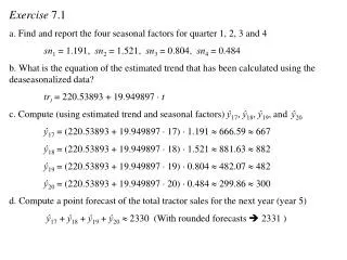
Exercise 7.1 a. Find and report the four seasonal factors for quarter 1, 2, 3 and 4 sn1 = 1.191, sn2 = 1.521, sn3 = 0.804, sn4 = 0.484 b. What is the equation of the estimated trend that has been calculated using the deaseasonalized data? trt = 220.53893 + 19.949897 t c. Compute (using estimated trend and seasonal factors) ŷ17, ŷ18, ŷ19, and ŷ20 ŷ17 = (220.53893 + 19.949897 17) 1.191 666.59 667 ŷ18 = (220.53893 + 19.949897 18) 1.521 881.63 882 ŷ19 = (220.53893 + 19.949897 19) 0.804 482.07 482 ŷ20 = (220.53893 + 19.949897 20) 0.484 299.86 300 d. Compute a point forecast of the total tractor sales for the next year (year 5) ŷ17 + ŷ18 + ŷ19 + ŷ20 2330 (With rounded forecasts 2331 )
e. Do the cyclical factors determine a well-defined cycle for these data? Explain your answer. Make a plot of cl together with cl ir In general the cycles would cover longer periods than a year, but this estimated cycle seems to have a period corresponding with four quarters. The answer is no.
f. In figure 7.5, find and report point forecasts of the tractor sales (based on trend and seasonal factors) for each of the quarters of next year (year 5). Do the values agree with your answers to part (c) ? g. (This is the task of assignment 2) h. Figure 7.6 (page 342) presents the MINITAB output of the 95% prediction interval forecasts of the deseasonalized tractor sales for each of the four quarters of the next year (year 5). use the results in this output to compute approximate 95% prediction interval forecasts of tractor sales for each of the quarters of the next year. Yes!
Quarter 17: 95% P.I. for y17* = d17 : (545.64, 573.76) See p. 339 in the textbook Error bound: (573.76 – 545.64)/2 = 14.06 Approx. 95% P.I. for y17 : (666.59 – 14.06, 666.59 + 14.06 ) (653, 681) Analogously for quarters 18-20: Error bound of P:I: for d18 : (594.00 – 565.31)/2 = 14.345 Approx 95% P.I. for y18: (867, 896) Error bound of P:I: for d19 : (614.26 – 584.94)/2 = 14.66 Approx 95% P.I. for y19: (467, 498) Error bound of P:I: for d20 : (634.55 – 604.55)/2 = 15 Approx 95% P.I. for y20: (285, 315)
Exercise 7.3 (Refer to Excel Worksheet, proceed as with 7.1) a. Find and report the four seasonal factors for quarter 1, 2, 3 and 4 sn1 = 70.59, sn2 = 210.76, sn3 = –76.95, sn4 = –204.41 b. What is the equation of the estimated trend that has been calculated using the deaseasonalized data? trt = 214.8895833 + 19.75563725 t c. Compute (using estimated trend and seasonal factors) ŷ17, ŷ18, ŷ19, and ŷ20 ŷ17 = (214.8895833 + 19.75563725 17) +70.59 621.33 621 ŷ18 = (214.8895833 + 19.75563725 18) + 210.76 781.25 781 ŷ19 = (214.8895833 + 19.75563725 19) – 76.95 513.30 513 ŷ20 = (214.8895833 + 19.75563725 20) – 204.41 405.59 406 d. Compute a point forecast of the total tractor sales for the next year (year 5) ŷ17 + ŷ18 + ŷ19 + ŷ20 2321 (With rounded forecasts 2321 )
e. Do the cyclical factors determine a well-defined cycle for these data? Explain your answer. Make a plot of cl together with cl ir No differences compared to the multiplicative case.
f. In figure 7.5, find and report point forecasts of the tractor sales (based on trend and seasonal factors) for each of the quarters of next year (year 5). Do the values agree with your answers to part (c) ? g. (This is the task of assignment 2) h. Figure 7.6 (page 342) presents the MINITAB output of the 95% prediction interval forecasts of the deseasonalized tractor sales for each of the four quarters of the next year (year 5). use the results in this output to compute approximate 95% prediction interval forecasts of tractor sales for each of the quarters of the next year. To be able to do the corresponding for the additive mode, we need a new Minitab (or SPSS or Eviews) analysis Yes!
The regression equation is d = 215 + 19.8 t Predictor Coef SE Coef T P Constant 214.89 20.08 10.70 0.000 t 19.756 2.076 9.52 0.000 S = 38.2841 R-Sq = 86.6% R-Sq(adj) = 85.7% Predicted Values for New Observations New Obs Fit SE Fit 95% CI 95% PI 1 550.74 20.08 (507.68, 593.79) (458.02, 643.45) 2 570.49 21.92 (523.47, 617.51) (475.87, 665.11) 3 590.25 23.81 (539.18, 641.31) (493.55, 686.94) 4 610.00 25.72 (554.83, 665.17) (511.08, 708.93)
Quarter 17: 95% P.I. for y17* = d17 : (458.02, 643.45) See p. 339 in the textbook Error bound: (643.45 – 458.02)/2 = 92.715 Approx. 95% P.I. for y17 : (621.33 – 92.715, 621.33 + 92.715 ) (529, 714) Analogously for quarters 18-20: Error bound of P:I: for d18 : (665.11 – 475.87)/2 = 94.62 Approx 95% P.I. for y18: (687, 876) Error bound of P:I: for d19 : (686.94 – 493.55)/2 = 96.695 Approx 95% P.I. for y19: (417, 610) Error bound of P:I: for d20 : (708.93 – 511.08)/2 = 98.925 Approx 95% P.I. for y20: (307, 505)
Does this method seem more appropriate for these data than the multiplicative method? Time series graph from Excel Workbook: Seasonal variation increases with level Support for the multiplicative model Prediction intervals much wider with additive model Strong support for the multiplicative model