Download
1 / 83
970 likes | 1.51k Views
Rietveld Refinement with GSAS. Recent Quote seen in Rietveld e-mail:. “Rietveld refinement is one of those few fields of intellectual endeavor wherein the more one does it, the less one understands.” (Sue Kesson). Stephens’ Law – “A Rietveld refinement is never perfected, merely abandoned”.

E N D
Rietveld Refinement with GSAS Recent Quote seen in Rietveld e-mail: “Rietveld refinement is one of those few fields of intellectual endeavor wherein the more one does it, the less one understands.” (Sue Kesson) Stephens’ Law – “A Rietveld refinement is never perfected, merely abandoned” Demonstration – refinement of fluroapatite R.B. Von Dreele, Advanced Photon Source Argonne National Laboratory
Rietveld refinement is multiparameter curve fitting • Result from fluoroapatite refinement – powder profile is curve with counting noise & fit is smooth curve • NB: big plot is sqrt(I) (lab CuKa B-B data) ) Iobs+ Icalc| Io-Ic| Refl. positions
So how do we get there? • Beginning – model errors misfits to pattern • Can’t just let go all parameters – too far from best model (minimum c2) False minimum Least-squares cycles c2 True minimum – “global” minimum parameter c2 surface shape depends on parameter suite
Fluoroapatite start – add model (1st choose lattice/sp. grp.) • important – reflection marks match peaks • Bad start otherwise – adjust lattice parameters (wrong space group?)
2nd add atoms & do default initial refinement – scale & background • Notice shape of difference curve – position/shape/intensity errors
Errors & parameters? • position – lattice parameters, zero point (not common) - other systematic effects – sample shift/offset • shape – profile coefficients (GU, GV, GW, LX, LY, etc. in GSAS) • intensity – crystal structure (atom positions & thermal parameters) - other systematic effects (absorption/extinction/preferred orientation) NB – get linear combination of all the above NB2 – trend with 2Q (or TOF) important peak shift wrong intensity too sharp LX - too small a – too small Ca2(x) – too small
Difference curve – what to do next? • Dominant error – peak shapes? Too sharp? • Refine profile parameters next (maybe include lattice parameters) • NB - EACH CASE IS DIFFERENT • Characteristic “up-down-up” • profile error NB – can be “down-up-down” for too “fat” profile
Result – much improved! • maybe intensity differences left – refine coordinates & thermal parms.
Result – essentially unchanged Ca F PO4 • Thus, major error in this initial model – peak shapes
So how does Rietveld refinement work? Rietveld Minimize Exact overlaps - symmetry Residuals: Io Incomplete overlaps SIc Ic Extract structure factors: Apportion Io by ratio of Ic to Sic & apply corrections
Rietveld refinement - Least Squares Theory Given a set of observations Gobs and a function then the best estimate of the values pi is found by minimizing This is done by setting the derivative to zero Results in n “normal” equations (one for each variable) - solve for pi
Least Squares Theory - continued Problem - g(pi) is nonlinear & transcendental (sin, cos, etc.) so can’t solve directly Expand g(pi) as Taylor series & toss high order terms ai - initial values of pi Dpi = pi - ai (shift) Substitute above Normal equations - one for each Dpi; outer sum over observations Solve for Dpi - shifts of parameters, NOT values
Least Squares Theory - continued Rearrange . . . Matrix form: Ax=v
Least Squares Theory - continued Matrix equation Ax=v Solve x = A-1v = Bv; B = A-1 This gives set of Dpi to apply to “old” set of ai repeat until all xi~0 (i.e. no more shifts) Quality of fit – “c2” = M/(N-P) 1 if weights “correct” & model without systematic errors (very rarely achieved) Bii = s2i – “standard uncertainty” (“variance”) in Dpi (usually scaled by c2) Bij/(Bii*Bjj) – “covariance” between Dpi & Dpj Rietveld refinement - this process applied to powder profiles Gcalc - model function for the powder profile (Y elsewhere)
Rietveld Model: Yc = Io{SkhF2hmhLhP(Dh) + Ib} Least-squares: minimize M=Sw(Yo-Yc)2 Io - incident intensity - variable for fixed 2Q kh - scale factor for particular phase F2h - structure factor for particular reflection mh - reflection multiplicity Lh - correction factors on intensity - texture, etc. P(Dh) - peak shape function - strain & microstrain, etc. Ib - background contribution
Peak shape functions – can get exotic! Convolution of contributing functions Instrumental effects Source Geometric aberrations Sample effects Particle size - crystallite size Microstrain - nonidentical unit cell sizes
2 1 2 2 ) = = L P ( D [ - 4 l n 2 D / H ] 4 l n 2 2 p H 2 k P ( D ) = e = G k k / H 1 + 4 D k H p k k k k CW Peak Shape Functions – basically 2 parts: Gaussian – usual instrument contribution is “mostly” Gaussian Lorentzian – usual sample broadening contribution • H - full width at half maximum - expression • from soller slit sizes and monochromator • angle • - displacement from peak position Convolution – Voigt; linear combination - pseudoVoigt
CW Profile Function in GSAS Thompson, Cox & Hastings (with modifications) Pseudo-Voigt Mixing coefficient FWHM parameter
CW Axial Broadening Function Finger, Cox & Jephcoat based on van Laar & Yelon Debye-Scherrer cone 2Q Scan H Slit 2QBragg 2Qmin 2Qi Depend on slit & sample “heights” wrt diffr. radius H/L & S/L - parameters in function (typically 0.002 - 0.020) Ä Pseudo-Voigt (TCH) = profile function
How good is this function? Protein Rietveld refinement - Very low angle fit 1.0-4.0° peaks - strong asymmetry “perfect” fit to shape
Bragg-Brentano Diffractometer – “parafocusing” Focusing circle X-ray source Diffractometer circle Receiving slit Incident beam slit Sample displaced Sample transparency Beam footprint Divergent beam optics
CW Function Coefficients - GSAS Shifted difference Sample shift Sample transparency Gaussian profile Lorentzian profile (plus anisotropic broadening terms) Intrepretation?
b* a* Crystallite Size Broadening Dd*=constant Lorentzian term - usual K - Scherrer const. Gaussian term - rare particles same size?
b* a* Microstrain Broadening Lorentzian term - usual effect Gaussian term - theory? Remove instrumental part
Microstrain broadening – physical model Model – elastic deformation of crystallites Stephens, P.W. (1999). J. Appl. Cryst. 32, 281-289. Also see Popa, N. (1998). J. Appl. Cryst. 31, 176-180. d-spacing expression Broadening – variance in Mhkl
Microstrain broadening - continued Terms in variance Substitute – note similar terms in matrix – collect terms
Microstrain broadening - continued Broadening – as variance 3 collected terms General expression – triclinic – 15 terms Symmetry effects – e.g. monoclinic (b unique) – 9 terms Cubic – m3m – 2 terms
Example - unusual line broadening effects in Na parahydroxybenzoate Sharp lines Broad lines Directional dependence - Lattice defects? Seeming inconsistency in line broadening - hkl dependent
H-atom location in Na parahydroxybenzoate Good DF map allowed by better fit to pattern DF contour map H-atom location from x-ray powder data
Macroscopic Strain Part of peak shape function #5 – TOF & CW d-spacing expression; aij from recip. metric tensor Elastic strain – symmetry restricted lattice distortion TOF: ΔT = (d11h2+d22k2+d33l2+d12hk+d13hl+d23kl)d3 CW: ΔT = (d11h2+d22k2+d33l2+d12hk+d13hl+d23kl)d2tanQ Why? Multiple data sets under different conditions (T,P, x, etc.)
Symmetry & macrostrain dij – restricted by symmetry e.g. for cubic DT = d11h2d3 for TOF Result: change in lattice parameters via change in metric coeff. aij’ = aij-2dij/C for TOF aij’ = aij-(p/9000)dij for CW Use new aij’ to get lattice parameters e.g. for cubic
L h Nonstructural Features Affect the integrated peak intensity and not peak shape Bragg Intensity Corrections: Extinction Preferred Orientation Absorption & Surface Roughness Other Geometric Factors
1 E = 1 + x b 2 3 x x 5 x E = 1 - + - . . . x < 1 2 4 4 8 l 2 1 3 é ù E = 1 - - . . . x > 1 p x ê ú 8 x 2 l 1 2 8 x ë û 2 2 E = E s i n Q + E c o s Q h b l Extinction Sabine model - Darwin, Zachariasen & Hamilton Bragg component - reflection Laue component - transmission Combination of two parts
80% E x 60% 40% 20% 0% 0.0 25.0 50.0 75.0 100.0 125.0 150.0 Sabine Extinction Coefficient Crystallite grain size = Increasing wavelength (1-5 Å) Eh 2Q
What is texture? Nonrandom crystallite grain orientations Random powder - all crystallite orientations equally probable - flat pole figure Pole figure - stereographic projection of a crystal axis down some sample direction Loose powder (100) random texture (100) wire texture Crystallites oriented along wire axis - pole figure peaked in center and at the rim (100’s are 90º apart) Orientation Distribution Function - probability function for texture Metal wire
Texture - measurement by diffraction (220) Non-random crystallite orientations in sample (200) Incident beam x-rays or neutrons Sample (111) • Debye-Scherrer cones • uneven intensity due to texture • also different pattern of unevenness for different hkl’s • Intensity pattern changes as sample is turned
Preferred Orientation - March/Dollase Model Uniaxial packing Ellipsoidal Distribution - assumed cylindrical Ro - ratio of ellipsoid axes = 1.0 for no preferred orientation Ellipsoidal particles Spherical Distribution Integral about distribution - modify multiplicity
l l ¥ m n m n å å å f ( g ) = C T ( g ) l l l=0 m=-l n=-l F1 F2 Y Texture - Orientation Distribution Function - GSAS Probability distribution of crystallite orientations - f(g) f(g) = f(F1,Y,F2) Tlmn = Associated Legendre functions or generalized spherical harmonics F1,Y,F2 - Euler angles
Texture effect on reflection intensity - Rietveld model • Projection of orientation distribution function for chosen reflection (h) and sample direction (y) • K - symmetrized spherical harmonics - account for sample & crystal symmetry • “Pole figure” - variation of single reflection intensity as fxn. of sample orientation - fixed h • “Inverse pole figure” - modification of all reflection intensities by sample texture - fixed y - Ideally suited for neutron TOF diffraction • Rietveld refinement of coefficients, Clmn, and 3 orientation angles - sample alignment
Absorption X-rays - independent of 2Q - flat sample – surface roughness effect - microabsorption effects - but can change peak shape and shift their positions if small (thick sample) Neutrons - depend on 2Q and l but much smaller effect - includes multiple scattering much bigger effect - assume cylindrical sample Debye-Scherrer geometry
Model - A.W. Hewat For cylinders and weak absorption only i.e. neutrons - most needed for TOF data not for CW data – fails for mR>1 GSAS – New more elaborate model by Lobanov & alte de Viega – works to mR>10 Other corrections - simple transmission & flat plate
Surface Roughness – Bragg-Brentano only Low angle – less penetration (scatter in less dense material) - less intensity High angle – more penetration (go thru surface roughness) - more dense material; more intensity Nonuniform sample density with depth from surface Most prevalent with strong sample absorption If uncorrected - atom temperature factors too small Suortti model Pitschke, et al. model (a bit more stable)
2 1 + M c o s 2 Q L = 2 p 2 s i n Q c o s Q 1 L = 2 p 2 s i n Q c o s Q 4 L = d s i n Q p Other Geometric Corrections Lorentz correction - both X-rays and neutrons Polarization correction - only X-rays X-rays Neutrons - CW Neutrons - TOF
Carbon scattering factor uncorrected 6 4 fC Solvent corrected 2 0 0 5 10 15 20 2Q Solvent scattering – proteins & zeolites? Contrast effect between structure & “disordered” solvent region f = fo-Aexp(-8pBsin2Q/l2) Babinet’s Principle: Atoms not in vacuum – change form factors
Background scattering Manual subtraction – not recommended - distorts the weighting scheme for the observations& puts a bias in the observationsFit to a function - many possibilities: Fourier series - empirical Chebyschev power series - ditto Exponential expansions - air scatter & TDS Fixed interval points - brute force Debye equation - amorphous background (separate diffuse scattering in GSAS)
Debye Equation - Amorphous Scattering real space correlation functionespecially good for TOFterms with vibration amplitude distance
Rietveld Refinement with Debye Function O 1.60Å 4.13Å Si 2.63Å 3.12Å 5.11Å 6.1Å a-quartz distances 7 terms Ri –interatomic distances in SiO2 glass 1.587(1), 2.648(1), 4.133(3), 4.998(2), 6.201(7), 7.411(7) & 8.837(21) Same as found in a-quartz
Non-Structural Features in Powder Patterns Summary 1. Large crystallite size - extinction 2. Preferred orientation 3. Small crystallite size - peak shape 4. Microstrain (defect concentration) 5. Amorphous scattering - background
Time to quit? Stephens’ Law – “A Rietveld refinement is never perfected, merely abandoned” Also – “stop when you’ve run out of things to vary” What if problem is more complex? Apply constraints & restraints “What to do when you have too many parameters & not enough data”