Download
1 / 18
180 likes | 192 Views
Learn the significance of variation interpretation, standard deviation calculation, and z-score computation. Discover the Greek symbols for mean and standard deviation, and explore the use of variance. Understand the importance of using SD with symmetrical data and the implications of skewed distributions. Gain insights into describing spread, normal distributions, and statistical tools. Take a closer look at the calculation process of standard deviation and variance. Enhance your grasp of variability measurement in datasets.

E N D
Learning Objectives By the end of this lecture, you should be able to: • Describe the importance that variation plays in interpreting a distribution • Understand how the standard deviation is calculated • Describe what is meant by a z-score and be able to calculate them • Start learning Greek: Be comfortable with the Greek letters for mean and standard deviation.
Another way of describing variation • Recall that perhaps the most succinct way summarize a distribution is in terms of its shape, center, and spread. • One method of summarizing the spread has already been discussed: Quartiles and the related 5-number summary. • Another extremely important method of describing spread is the ‘variance’ or ‘standard deviation’. • Variance and SD are essentially the same thing. The standard deviation is simply the square root of the variance. • E.g.: If Variance is 25, then SD = 5. If SD = 7, then Variance = 49. • When 'interpreting' statistical data, or explaining a distribution, people tend to use standard deviation. • For theoretical application and development, variance is typically used. • We will typically use SD in this course. • Generally, you should only use Variance / SD with data that has a symmetrical distribution • That is, using SD/Variance to describe spread can lead to inaccurate calculations if looking at data that is NOT normally distributed. This is important! • The reason is that in order to calculate the SD, we need to use the mean of that data. • Terminology review: We say that the SD is not resistant to skewed data.
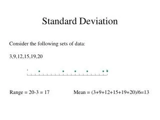
Variation In every set of values (“dataset”—know this term!) e.g. ages, heights, incomes, crop yields, spitball-distances, etc. there will always be variation. The question is, how do we describe just how varied our data is? Are all the points closely clustered around some value or are they all over the map? Having a sense of how much the various datapoints are spread out around the center (mean or median) is an important piece of information. Consider employee pay at DePaul University: if we looked at every income from student workers to the Provost/President, we would see a tremendous variation around the center as some people make a great deal more than the center, and some make much less. However, if we focused only on student employees, we would find that the variation around the center is considerably less. Suppose we were looking at a widget used in the construction of a high-performance laser. Suppose this widget is intended to be exactly 2.3 inches in diameter. A manufacturer must make their parts extremely close to this diameter in order for them to fit properly. We would assume that the average diameter of, say, 10000 parts would indeed be very close to 2.3. However, the question from a manufacturing perspective would be: How much variation is there among the parts? The manufacturer would hope that the variation would be extremely small, that is, nearly all the parts are very close in size to the mean. If there is a large variation, it would mean that there are several parts that are inappropriately sized, and many of our very expensive lasers are going to be faulty. The most common statistic we used for measuring variability (spread) is called the standard deviation.
How to calculate the SD (Note: This is for explanatory purposes only - you will not have to do this by hand) Find the mean (e.g. 63.5) Look at one datapoint (e.g. 63) and calculate its difference from the mean. (e.g. -0.5) Square it that value (0.25). Repeat for all datapoints. Then add up all values from step 3. Divide by n-1 ('n' equals the number of observations) You now have the variance. To get from variance to SD, simply take the square root of the variance.
Calculating standard deviation: ‘s’ Women height (inches) Calculating these by hand can be tedious. We may do a couple of examples, but will quickly switch over to doing them using a computer. • Mean = 63.4 • Sum of squared deviations from mean = 85.2 • Degrees freedom (df) = (n − 1) = 13 • s2 = variance = 85.2 / 13 = 6.55 inches2 • s = standard deviation = √6.55 = 2.56 inches
Review: Why do we care so much about Normal distributions? • Much of the data we examine in the real world turns out to have a normal distribution (exam scores, survival length for cancer patients, crop yields, SAT results, people’s heights, birth rate of rabbits, games of chance, etc., etc., etc.) • As a result, a great deal of study and research has gone into the properties of Normal distributions/curves, as a result of which, we have many tools that we can use to come up with statistics for analysis of our data. • In fact, some of the various tools discussed in this lecture (standard deviation, z-score, z-tables) usually apply only to Normal distributions.
Calculating areas under the Normal curve • Recall how in a previous discussion, we calculated probabilities by estimating the areas under the Normal density curve. • The standard deviation is a number we can use to accuratelydetermine the area under any segment of the Normal curve. We will discuss this over the next couple of lectures. What percentage of test takers would be expected to score below 6.0?
Overview of determining the area under the curve A fairly straight-forward process: Using the standard deviation, convert the value you are interested in (e.g. in this case, a Grade equivalent score of 6.0) into something called a z-score. Look up your z-score in a normal probability table (also called a z-table) The value you find on the z-table, is the area under the curve to the left of your score (e.g. 6.0). While you should spend a few minutes thinking about this slide, don’t worry too much about it for now. We will revisit it later. What percentage of test takers would be expected to score below 6.0?
The z-score • Know the following two facts: • A z-score measures the number of standard deviations that some value ‘x’ is from the mean. • E.g. a z-score of +1.0 means the value lies 1 standard deviation above the mean. • E.g. a z-score of +0.5 means the value lies one-half standard deviation above the mean. • E.g. a z-score of -1.23 means the value lies 1.23 standard deviations below the mean. • As long as you know the SD, any observation can be converted to a z-score. • That is, every observation can be converted into a z-score, and any z-score can be converted back to an observation. • You should be very comfortable with this concept!
It’s all Greek to me … And it’s gonna get a little worse. But we’ll start slow… • In the math world, there are numerous ‘shortcuts’ that are used to represent certain concepts. • Such symbols are both widespread and useful (though I believe sometimes it's just geeks trying to look impressive). • However, you must get comfortable with them as they are introduced. • Here are two to begin with: • μ (mu) mean of a values from a population • σ (sigma) standard deviation of values from a population
Practice: z-score using the GEQ (Grade Equivalent Score) dataset If I tell you that: Mean ( μ ) = 7, Standard Deviation (σ ) is 1: • Example: Your score is 6. How many standard deviations does your score lie above or below the mean? • Answer: z = -1. Your score is exactly 1 standard deviation below the mean. • Example: Your score is 8. How many standard deviations does your score lie above or below the mean? • Answer: z = +1. Your score is exactly 1 standard deviation above the mean. • Example: Your score is 5.5. How many standard deviations does your score lie above or below the mean? • Answer: z = -1.5. Your score is 1.5 standard deviations below the mean.
z-score = number of SDs • Recall that z-score is simply a value that tells us the number of standard deviations above or below the mean. • So if I ask you “How many SDs above or below the mean?” – that is exactly the same thing as asking you for “the z-score”. • If you are not clear on this concept, be sure to practice and review the previous slide.
Practice: z-score using the GEQ (Grade Equivalent Score) dataset Given: Mean ( μ ) = 7, Standard Deviation ( σ ) is 0.5 • Example: x = 6. How many standard deviations does this observation lie above or below the mean? I.e. What is the z-score? • Answer: z = -2. Your score is exactly 2 standard deviations below the mean. • Example: x = 8.5. What is the z-score? • Answer: z = +3. Your score is 3 standard deviations above the mean. • Example: x =5. What is the z-score? • Answer: z = -4. Your score is 4 standard deviations below the mean. • Example: x = 5.423. What is the z-score? • Answer: Uh-oh, this one is a bit trickier… See next slide.
Formula for calculating the z-score Most observations are not values that are exactly +1 or +2 or -1 or -2 (etc.) standard deviations away from the mean. Fortunately, there is a simple formula for accurately calculating a z-score. However, you should always keep in mind what it is you are calculating when you apply this formula. Do not ever forget that a z-scoremeasures the number of standard deviations that a data value x is from the mean m. • x the specific observation we are asking about • μ the mean of the population • σ the standard deviation of the population
Practice: z-score using the GEQ (Grade Equivalent Score) dataset Example: The distribution has μ = 7, σ = 0.5. Your child scored is 5.423. What is their z-score? • Answer: Use the formula: • So • x = 5.423 • μ = 7 • σ = 0.5 • Therefore: z = (5.423 – 7) / 0.5 z = -3.154 • In other words, our score is 3.154 standard deviations below the mean.
Example: Calculate the z-score for x = 200. μ = 197 and σ = 342. • Answer: Because this is not a Normal distribution, the mean and standard deviation are NOT good choices of statistics to use in an analysis. And without a mean and standard deviation, we can not calculate a z-score! • Take-home point: DON’T JUST THROW NUMBERS AT A FORMULA. THE CONCEPT IS THE KEY! In this case, recall that standard deviations should be avoided for distributions that are skewed and/or have outliers. • Another take-home point: Looking at a graph of your data is HUUUUGELY important!! If we hadn't done so, we would have been unaware that the data was skewed! Do not lose site of these two very important facts!!! This is possibly the most important point of the entire course!
Punching numbers into a calculator (or statistical software) is easy!! • It is ALWAYS possible to calculate a mean (and SD, and countless other statistics) of a dataset. However, just because you can punch numbers into a calculator or statistical software does not mean that those numbers mean anything useful! • In fact, quite the opposite. One of the most damaging mistakes people use when making decisions is applying a formula when that formula is not the right tool for the job. • One of the most important things I want you to take away from this entire course is the ability to distinguish the right tool for the job from the wrong tool for the job! This takes a little bit of review and practice of concepts, but it is absolutely doable!! • Recall from our first lectures that the mean is usually the WRONG tool for the center of a distribution if the distribution is skewed or has significant outliers. • In fact, you should ALWAYS try to see a graph of any data that you are attempting to analyze.