Quick Mapping with ggmap: Overlaying Lat/Long Data on Maps
Learn how to overlay latitude/longitude data on maps using ggmap library in R. Follow step-by-step guide with examples and tutorials.

Quick Mapping with ggmap: Overlaying Lat/Long Data on Maps
E N D
Presentation Transcript
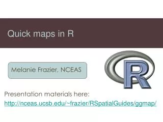
Quick maps in R Melanie Frazier, NCEAS Presentation materials here: http://nceas.ucsb.edu/~frazier/RSpatialGuides/ggmap/
Have Lat/Long data? And, you want to see where they are Data from the EPA’s WestuRe project: http://www.epa.gov/wed/pages/models/WestuRe/WestuRe.htm
Many options: But we’ll stick with 2 library(plotKML) library(ggmap)
ggmap Part 1 Download the map raster Part 2 Overlay data onto raster Refer to Quickstart guide:
ggmap: Part 1 (getting the map) Specify coordinates - geocode myLocation <- “University of Washington” - Lat/Long myLocation <- c(lon=-95.36, lat=29.76) - Bounding box (lowerleftlon, lowerleftlat, upperrightlon, upperrightlat) myLocation <- c(-130, 30, -105, 50) [NOTE: glitchy for google maps]
ggmap: Part 1 (getting the map) B. Define map source, maptype, and color maptype = watercolor toner terrain source stamen terrain satellite roadmap hybrid google color can do any of the maps in “bw” osm (and, cloudmade)
ggmap: Part 1 (getting the map) B. Define map source, maptype, and color Scale matters in regard to map source/type
ggmap: Part 1 (getting the map) B. get_mapfunction provides a general approach for quickly getting maps myMap <- get_map(location = myLocation, source = “stamen”, maptype = “watercolor”, color = “bw”) Additional options such as “zoom” and “crop” ?ggmap
ggmap: Part 1 (getting the map) Sometimes get_map doesn’t provide the control needed to get the map you want. In this case, use the specific functions designed for the different map sources: get_googlemap get_openstreetmap get_stamenmap get_cloudmademap
ggmap: Part 2 (overlaying your data) A. Plot the raster ggmap(myMap) B. Get your lat/long point data: myData <- read.csv(“http://nceas.ucsb.edu/~frazier/RSpatialGuides/ggmap/EstuaryData.csv”) C. Add points (ggplot2 syntax) ggmap(myMap)+ geom_point(aes(x=estLongitude, y=estLatitude), data=myData, alpha=0.5, color=“darkred”, size=3)
plotKML Tutorial: http://gsif.isric.org/doku.php?id=wiki:tutorial_plotkml Load libraries: library(plotKML) library(sp) Convert to spatial dataframe object: coordinates(myData) <- ~estLongitude+estLatitude Provide the projection (just copy this): proj4string(myData) <- CRS("+proj=longlat +datum=WGS84") Make the plot: plotKML(myData, colour="lnEstArea", balloon=TRUE)
Questions Presentation materials here: http://nceas.ucsb.edu/~frazier/RSpatialGuides/ggmap/