Download
1 / 8
80 likes | 105 Views
Explore Bayes's Rule, Bernoulli and Binomial random variables in a poker context. Learn how to calculate probabilities, expected values, and variances. Get ready for your midterm with this essential probability guide.

E N D
Stat 35b: Introduction to Probability with Applications to Poker Outline for the day: • Bayes’s Rule • Bernoulli random variables. • Binomial random variables. • Farha vs. Antonius, expected value and variance. • Midterm is Feb 21, in class. 50 min. • Open book plus one page of notes, double sided. Bring a calculator! u u
1. Bayes’s rule, p49-52. Suppose that B1, B2 , Bn are disjoint events and that exactly one of them must occur. Suppose you want P(B1 | A), but you only know P(A | B1 ), P(A | B2 ), etc., and you also know P(B1), P(B2), …, P(Bn). Bayes’ Rule: If B1 , …, Bn are disjoint events with P(B1 or … or Bn) = 1, then P(Bi | A) = P(A | Bi ) * P(Bi) ÷ [ ∑P(A | Bj)P(Bj)]. Why? Recall: P(X | Y) = P(X & Y) ÷ P(Y). So P(X & Y) = P(X | Y) * P(Y). P(B1 | A) = P(A & B1 ) ÷ P(A) = P(A & B1 ) ÷ [ P(A & B1) + P(A & B2) + … + P(A & Bn) ] = P(A | B1 ) * P(B1) ÷ [ P(A | B1)P(B1) + P(A | B2)P(B2) + … + P(A | Bn)P(Bn) ].
Bayes’s rule, continued. Bayes’s rule: If B1 , …, Bn are disjoint events with P(B1 or … or Bn) = 1, then P(Bi | A) = P(A | Bi ) * P(Bi) ÷ [ ∑P(A | Bj)P(Bj)]. See example 3.4.1, p50. If a test is 95% accurate and 1% of the pop. has a condition, then given a random person from the population, P(she has the condition | she tests positive) = P(cond | +) = P(+ | cond) P(cond) ÷ [P(+ | cond) P(cond) + P(+ | no cond) P(no cond)] = 95% x 1% ÷ [95% x 1% + 5% x 99%] ~ 16.1%. Tests for rare conditions must be extremely accurate.
Bayes’ rule example. Suppose P(your opponent has the nuts) = 1%, and P(opponent has a weak hand) = 10%. Your opponent makes a huge bet. Suppose she’d only do that with the nuts or a weak hand, and that P(huge bet | nuts) = 100%, and P(huge bet | weak hand) = 30%. What is P(nuts | huge bet)? P(nuts | huge bet) = P(huge bet | nuts) * P(nuts) ------------------------------------------------------------------------------------------- P(huge bet | nuts) P(nuts) + P(huge bet | horrible hand) P(horrible hand) = 100% * 1% --------------------------------------- 100% * 1% + 30% * 10% = 25%.
2. Bernoulli Random Variables, ch. 5.1. If X = 1 with probability p, and X = 0 otherwise, then X = Bernoulli (p). Probability mass function (pmf): P(X = 1) = p P(X = 0) = q, where p+q = 100%. If X is Bernoulli (p), then µ = E(X) = p, and s= √(pq). For example, suppose X = 1 if you have a pocket pair next hand; X = 0 if not. p = 5.88%. So, q = 94.12%. [Two ways to figure out p: (a) Out of choose(52,2) combinations for your two cards, 13 * choose(4,2) are pairs. 13 * choose(4,2) / choose(52,2) = 5.88%. (b) Imagine ordering your 2 cards. No matter what your 1st card is, there are 51 equally likely choices for your 2nd card, and 3 of them give you a pocket pair. 3/51 = 5.88%.] µ = E(X) = .0588. SD = s= √(.0588 * 0.9412) = 0.235.
3. Binomial Random Variables, ch. 5.2. Suppose now X = # of times something with prob. p occurs, out of n independent trials Then X = Binomial (n.p). e.g. the number of pocket pairs, out of 10 hands. Now X could = 0, 1, 2, 3, …, or n. pmf: P(X = k) = choose(n, k) * pk qn - k. e.g. say n=10, k=3: P(X = 3) = choose(10,3) * p3 q7 . Why? Could have 1 1 1 0 0 0 0 0 0 0, or 1 0 1 1 0 0 0 0 0 0, etc. choose(10, 3) choices of places to put the 1’s, and for each the prob. is p3 q7 . Key idea: X = Y1 + Y2 + … + Yn , where the Yi are independent and Bernoulli (p). If X is Bernoulli (p), then µ = p, and s= √(pq). If X is Binomial (n,p), then µ = np, and s= √(npq).
Binomial Random Variables, continued. Suppose X = the number of pocket pairs you get in the next 100 hands. What’s P(X = 4)? What’s E(X)? s? X = Binomial (100, 5.88%). P(X = k) = choose(n, k) * pk qn - k. So, P(X = 4) = choose(100, 4) * 0.0588 4 * 0.9412 96 = 13.9%, or 1 in 7.2. E(X) = np = 100 * 0.0588 = 5.88. s= √(100 * 0.0588 * 0.9412) = 2.35. So, out of 100 hands, you’d typically get about 5.88 pocket pairs, +/- around 2.35.
4) Farha vs. Antonius, expected value and variance. E(X+Y) = E(X) + E(Y). Whether X & Y are independent or not! Similarly, E(X + Y + Z + …) = E(X) + E(Y) + E(Z) + … And, if X & Y are independent, then V(X+Y) = V(X) + V(Y). so SD(X+Y) = √[SD(X)^2 + SD(Y)^2]. Also, if Y = 9X, then E(Y) = 9E(Y), and SD(Y) = 9SD(X). V(Y) = 81V(X). Farha vs. Antonius. Running it 4 times. Let X = chips you have after the hand. Let p be the prob. you win. X = X1 + X2 + X3 + X4, where X1 = chips won from the first “run”, etc. E(X) = E(X1) + E(X2) + E(X3) + E(X4) = 1/4 pot (p) + 1/4 pot (p) + 1/4 pot (p) + 1/4 pot (p) = pot (p) = same as E(Y), where Y = chips you have after the hand if you ran it once! But the SD is smaller: clearly X1 = Y/4, so SD(X1) = SD(Y)/4. So, V(X1) = V(Y)/16. V(X) ~ V(X1) + V(X2) + V(X3) + V(X4), = 4 V(X1) = 4 V(Y) / 16 = V(Y) / 4. So SD(X) = SD(Y) / 2.