Reinforcement Learning
550 likes | 569 Views
This presentation covers reinforcement learning in artificial intelligence, with a focus on Markov decision processes. Topics include search, constraint satisfaction problems, games, and value iteration. Learn how to find optimal policies and solve MDPs with value and policy iteration methods.

Reinforcement Learning
E N D
Presentation Transcript
Reinforcement Learning Tamara Berg CS 590-133 Artificial Intelligence Many slides throughout the course adapted from Svetlana Lazebnik, Dan Klein, Stuart Russell, Andrew Moore, Percy Liang, Luke Zettlemoyer
Announcements • HW1 is graded • Grades are in your submission folders in a file called grade.txt(mean = 14.15, median = 18) • Thursday we’ll have demos of extra-credits • Office hours canceled today
Reminder • Mid-term exam next Tuesday, Feb 18 • Held during regular class time in SN014 and SN011 • Closed book • Short answer written questions • Shubham will hold a mid-term review + Q&A session, Feb 14 at 5pm in SN 014.
Exam topics 1) Intro to AI, agents and environments Turing test Rationality Expected utility maximizationPEASEnvironment characteristics: fully vs. partially observable, deterministic vs. stochastic, episodic vs. sequential, static vs. dynamic, discrete vs. continuous, single-agent vs. multi-agent, known vs. unknown 2) SearchSearch problem formulation: initial state, actions, transition model, goal state, path cost State space Search tree Frontier Evaluation of search strategies: completeness, optimality, time complexity, space complexity Uninformed search strategies: breadth-first search, uniform cost search, depth-first search, iterative deepening search Informed search strategies: greedy best-first, A*, weighted A* Heuristics: admissibility, dominance
Exam topics 3) Constraint satisfaction problems Backtracking search Heuristics: most constrained/most constraining variable, least constraining value Forward checking, constraint propagation, arc consistencyTree-structured CSPsLocal search 4) GamesZero-sum games Game treeMinimax/Expectimax/ExpectiminimaxsearchAlpha-beta pruningEvaluation functionQuiescence searchHorizon effectStochastic elements in games
Exam topics 5) Markov decision processesMarkov assumption, transition model, policy Bellman equationValue iterationPolicy iteration 6) Reinforcement learning Model-based vs. model-free approaches Passive vs Active Exploration vs. exploitation Direct EstimationTD Learning TD Q-learning
Markov Decision Processes Stochastic, sequential environments Image credit: P. Abbeel and D. Klein
Markov Decision Processes • Components: • Statess, beginning with initial state s0 • Actionsa • Each state s has actions A(s) available from it • Transition model P(s’ | s, a) • Markov assumption: the probability of going to s’ from s depends only on s and a and not on any other past actions or states • Reward functionR(s) • Policy(s): the action that an agent takes in any given state • The “solution” to an MDP
Overview • First, we will look at how to “solve” MDPs, or find the optimal policy when the transition model and the reward function are known • Second, we will consider reinforcement learning, where we don’t know the rules of the environment or the consequences of our actions
Grid world Transition model: 0.1 0.8 0.1 R(s) = -0.04 for every non-terminal state Source: P. Abbeel and D. Klein
Goal: Policy Source: P. Abbeel and D. Klein
Grid world Transition model: R(s) = -0.04 for every non-terminal state
Grid world Optimal policy when R(s) = -0.04 for every non-terminal state
Grid world • Optimal policies for other values of R(s):
Solving MDPs • MDP components: • Statess • Actionsa • Transition model P(s’ | s, a) • Reward functionR(s) • The solution: • Policy(s): mapping from states to actions • How to find the optimal policy?
Finding the utilities of states Max node • What is the expected utility of taking action a in state s? • How do we choose the optimal action? Chance node P(s’ | s, a) U(s’) • What is the recursive expression for U(s) in terms of the utilities of its successor states?
The Bellman equation • Recursive relationship between the utilities of successive states: Receive reward R(s) Choose optimal action a End up here with P(s’ | s, a) Get utility U(s’) (discounted by )
The Bellman equation • Recursive relationship between the utilities of successive states: • For N states, we get N equations in N unknowns • Solving them solves the MDP • We can solve them algebraically • Two methods: value iteration and policy iteration
Method 1: Value iteration • Start out with every U(s) = 0 • Iterate until convergence • During the ith iteration, update the utility of each state according to this rule: • In the limit of infinitely many iterations, guaranteed to find the correct utility values • In practice, don’t need an infinite number of iterations…
Value iteration • What effect does the update have? Value iteration demo
Values vs Policy • Basic idea: approximations get refined towards optimal values • Policy may converge long before values do
Method 2: Policy iteration • Start with some initial policy 0 and alternate between the following steps: • Policy evaluation: calculate Ui(s) for every state s • Policy improvement: calculate a new policy i+1 based on the updated utilities
Policy evaluation • Given a fixed policy , calculate U(s) for every state s • The Bellman equation for the optimal policy: • How does it need to change if our policy is fixed? • Can solve a linear system to get all the utilities! • Alternatively, can apply the following update:
What is machine learning? • Computer programs that can learn from data • Two key components • Representation: how should we represent the data? • Generalization: the system should generalize from its past experience (observed data items) to perform well on unseen data items.
Types of ML algorithms • Unsupervised • Algorithms operate on unlabeled examples • Supervised • Algorithms operate on labeled examples • Semi/Partially-supervised • Algorithms combine both labeled and unlabeled examples
Types of ML algorithms • Unsupervised • Algorithms operate on unlabeled examples • Supervised • Algorithms operate on labeled examples • Semi/Partially-supervised • Algorithms combine both labeled and unlabeled examples
Example: Image classification input desired output apple pear tomato cow dog horse Slide credit: Svetlana Lazebnik
http://yann.lecun.com/exdb/mnist/index.html Slide from Dan Klein
Reinforcement learning for flight • Stanford autonomous helicopter
Types of ML algorithms • Unsupervised • Algorithms operate on unlabeled examples • Supervised • Algorithms operate on labeled examples • Semi/Partially-supervised • Algorithms combine both labeled and unlabeled examples
Supervised learning has many successes • recognize speech, • steer a car, • classify documents • classify proteins • recognizing faces, objects in images • ... Slide Credit: AvrimBlum
However, for many problems, labeled data can be rare or expensive. Unlabeled data is much cheaper. Need to pay someone to do it, requires special testing,… Slide Credit: AvrimBlum
However, for many problems, labeled data can be rare or expensive. Unlabeled data is much cheaper. Need to pay someone to do it, requires special testing,… SpeechImagesMedical outcomes Customer modelingProtein sequencesWeb pages Slide Credit: AvrimBlum
However, for many problems, labeled data can be rare or expensive. Unlabeled data is much cheaper. Need to pay someone to do it, requires special testing,… [From Jerry Zhu] Slide Credit: AvrimBlum
However, for many problems, labeled data can be rare or expensive. Unlabeled data is much cheaper.Can we make use of cheap unlabeled data? Need to pay someone to do it, requires special testing,… Slide Credit: AvrimBlum
But unlabeled data is missing the most important info!! But maybe still has useful regularities that we can use. Semi-Supervised Learning Canweuseunlabeleddatatoaugment a smalllabeledsampletoimprovelearning? But… But… But… Slide Credit: AvrimBlum
Reinforcement Learning • Components (same as MDP): • Statess, beginning with initial state s0 • Actionsa • Each state s has actions A(s) available from it • Transition model P(s’ | s, a) • Reward functionR(s) • Policy(s): the action that an agent takes in any given state • The “solution” • New twist: don’t know Transition model or Reward function ahead of time! • Have to actually try actions and states out to learn
Reinforcement learning: Basic scheme • In each time step: • Take some action • Observe the outcome of the action: successor state and reward • Update some internal representation of the environment and policy • If you reach a terminal state, just start over (each pass through the environment is called a trial) • Why is this called reinforcement learning?
Passive Reinforcement learning strategies • Model-based • Learn the model of the MDP (transition probabilities and rewards) and evaluate the state utilities under the given policy • Model-free • Learn state utilities without explicitly modeling the transition probabilities P(s’ | s, a) • TD-learning: use the observed transitions and rewards to adjust the utilities of states so that they agree with the Bellman eqns
