Download
1 / 48
480 likes | 505 Views
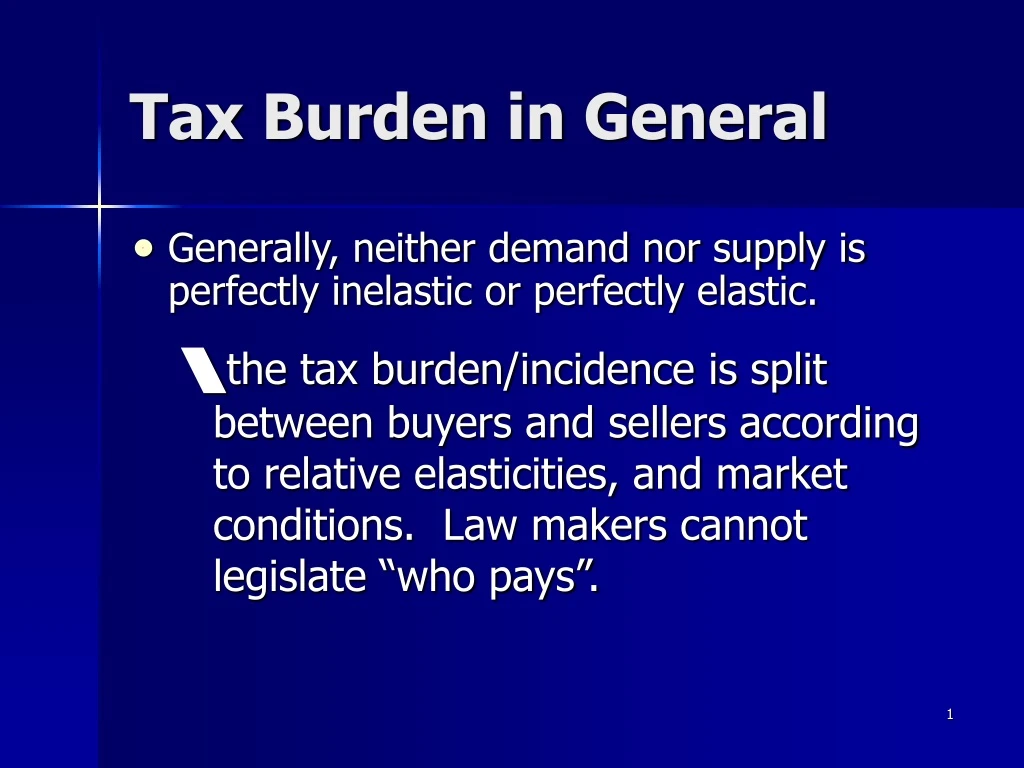
Tax Burden in General. Generally, neither demand nor supply is perfectly inelastic or perfectly elastic. the tax burden/incidence is split between buyers and sellers according to relative elasticities, and market conditions. Law makers cannot legislate “who pays”. Addiction and Elasticity.

E N D
Tax Burden in General • Generally, neither demand nor supply is perfectly inelastic or perfectly elastic. \the tax burden/incidence is split between buyers and sellers according to relative elasticities, and market conditions. Law makers cannot legislate “who pays”.
Addiction and Elasticity • Nonusers’ demand for addictive substances is elastic. • High taxes on cigarettes and alcohol limit the number of young people who become habitual users of these products. • Existing users’ demand for addictive substances is inelastic. • High taxes have only a modest effect on the quantities consumed by established user, they raise revenue from these users.
Luxury Tax • Notice that depending on the goal of the tax different types of demand elasticity are desirable. • Raise revenue: inelastic demand • Change behaviour: elastic demand • Who actually bore the burden of this tax?
Tax Burden and Elasticity of Demand • Two extreme cases: • Perfectly inelastic demand: • Perfectly elastic demand: Tax Burden and Elasticity of Supply • Two extreme cases: • Perfectly inelastic supply: • Perfectly elastic supply:
Sales Tax and the Elasticity of Demand S’ Tax S 2.20 Perfectly inelastic demand Price (dollars per dose) 2.00 Buyer pays entire tax D 100 Quantity (thousands of doses per day)
Sales Tax and the Elasticity of Demand S’ S D 1.00 Tax Price (cents per pen) Perfectly elastic demand 0.90 Seller pays entire tax 4 Quantity (thousands of marker pens per week)
Sales Tax and the Elasticity of Supply S Perfectly inelastic supply 50 Price (dollars per bottle) Seller paysentire tax Tax 45 D 100 Quantity (thousands of bottles per week)
Sales Tax and the Elasticity of Supply Perfectly Elastic Supply Price (cents per pound) S’ 11 Buyer paysentire tax Tax 10 S D 3 5 Quantity (thousands of kilograms per week)
Who pays the Airport Security Tax? • Who pays the tax? - Demand Elasticity between 0.7 and 2.1 • No mention of elasticity of supply but economists claim the price will rise by the amount of the tax, • Ie: the buyer pays the whole tax, implying a perfectly elastic supply schedule.
S+tax 950 1,230 Supply: Perfectly Elastic Original Equilibrium P=$60, Q=1,400 passengers/day Elasticity of Demand = 2.1 100 Elasticity of Demand = 0.7 80 72 Price (dollars per trip) 60 S D1 40 20 D0 1,400 2,100 Quantity (passengers per day)
S+tax 1,290 1,220 Supply: Unit Elastic Elasticity of Demand = 2.1 100 Elasticity of Demand = 0.7 80 S Price (dollars per trip) 60 40 D1 20 Crucial to know demand elasticity & supply elasticity D0 2,100 1,400 Quantity (passengers per day)
S2 Rent ceiling Housing shortage Housing shortage A Rent Ceiling & Elasticity S1, SR Supply in the LR becomes more elastic over time, increasing the shortage 24 20 Rent (dollars per unit per month) 16 D 12 0 44 72 100 150 Quantity(thousands of units per month)
How Long is the Long Run? • There is no set amount of time that puts a market into the long run • The long run could be a week or a year • The long run is how long a consumer or firm takes to fully adjust to a price change • Time required to make major changes • Ie) Give up Pepsi Vanilla, Build more cost efficient Pepsi factory, secure a US Pepsi Vanilla supplier • The short run is anything shorter than the long run
Cross Price Elasticity of Demand • We’ve seen already that demand is affected by the price of substitutes and compliments • An increase in the price of a substitute increases demand • An increase in the price of a complement decrease demand • This effect can be measured using cross price elasticity • If the cross price elasticity is zero, the good is neither a complement nor a substitute
Percentage change in quantity demanded of X E xy Percentage change in price of Y Cross Price Elasticity of Demand Exy = Change in X --------------- (X1 + X2)/2 / Change in Price of Y ---------------------------- (Py1 + Py2)/2 Substitutes – Positive Cross Price Elasticity Compliments – Negative Cross Price Elasticity
Income Elasticity of Demand • Income Elasticity of demand refers to a HORIZONTAL SHIFT in the demand curve resulting from an income change • Price elasticity of demand refers to a MOVEMENT ALONG THE DEMAND CURVE in response to a price change
Percentage change in quantity demanded E xy Percentage change in income Income Elasticity of Demand EI= Change in Q --------------- (Q1 + Q2)/2 / Change in M ---------------------------- (M1 + M2)/2 Normal Good – Positive Shift/Elasticity Inferior Good – Negative Shift/Elasticity
The Theory of Consumer Choice • The theory of consumer choice attempts to explain why consumers choose one good or bundle of goods over another good or bundle of goods.
The Theory of Consumer Choice • We are particularly interested in how prices affect consumer choice (demand) because • making choices in response to prices and price changes is the basis of the operation of the price system. • Cet. Par.
“Measuring” Satisfaction • util: unit of pleasure. • utility: a number that represents the level of satisfaction that the consumer derives from consuming a specific quantity of a good.
Trips to Club Total utility Marginal utility 1 2 3 4 5 6 12 22 28 32 34 34 12 10 6 4 2 0 Total Utility, Marginal Utility Frank’s TU & MU from country music: Total utility & marginal utility of trips to the club per week • TU (total utility): • the total amount of satisfaction that you get from consuming a product. • MU (marginal utility): • the increase in TU that comes about as a result of consuming one more unit of the product.
Marginal Utility • If one more unit of a good is consumed, the marginal utility is equal to the increased utility from that extra good • If more than one additional good is consumed:
Total utility is maximized... 34 28 Total Utility (utils per week) 22 0 2 3 4 5 6 7 8 …where marginal utility equals zero. Performances per Week Total and Marginal Utility of Club Trips 10 8 6 Marginal Utility (utils per week) 4 2 0 7 2 3 4 5 6 Performances per Week
Law of Diminishing MU • The MU (marginal utility) of a good or service will decline as more units of that good or service are consumed. • Marginal utility is what counts for rational consumer decisions.
Frank’s Optimal Choice • When Frank can go to each activity for free, he splits his time between the two to maximize utility. At each successive step, he chooses the activity with the greatestMU.
(1) Per week (2) Total utility (3) Marginal utility (MU) 12 22 28 32 34 34 12 10 06 04 02 00 1 2 3 4 5 6 Trips to club 1 2 3 4 5 6 21 33 42 48 51 51 21 12 09 06 03 00 Basketball games
Frank’s Optimal Choice • _night club visits and _ nights at basketball • for a total satisfaction = __ utils. • In the real world, Frank cannot have whatever he wants, he must maximize utility subject to: 1.) the income constraint 2.) the nature of commodity prices
Rational Choice Spend limited income where satisfaction per $ is the greatest. • MU/$: marginal benefit of the decision. • MU/$: marginal cost of the next best alternative given up choose those items for which MU/$ is the greatest until all income is spent.
Frank’s Optimal Decision • Suppose: Frank has an entertainment • budget of $21.00 • club tickets $3.00 • basketball tickets $6.00 • Under these circumstances, the best Frank can do is 1.) allocate (spend) all his income so that 2.) MU basketball = MU club trips P basketball P club trips
(3) Marginal Utility (MU) (5) Marginal Utility/$ (MU/P) (2) Total Utility (4) Price (P)$ (1) per week 1 2 3 4 5 6 12 22 28 32 34 34 12 10 06 04 02 00 3.00 3.00 3.00 3.00 3.00 3.00 4.0 3.3 2.0 1.3 0.7 0.0 Trips to Club Income = $21 Pc = $3.00 Pb = $6.00 1 2 3 4 5 6 21 33 42 48 51 51 21 12 09 06 03 00 6.00 6.00 6.00 6.00 6.00 6.00 3.5 2.0 1.5 1.0 0.5 0.0 B’ball games per/wk
Frank’s Optimal Decision The rational consumer will choose a “market basket” where the MU of the last $ spent on all commodities is the same and all income is spent. • Why does this maximize utility?
Frank’s Optimal Decision Suppose, Frank buys 3 basketball games and 1 club trip MUBB = 1.5 MU club = 4 PBB P club MBc > MCb • Frank is better off to take another club trip and give up one basketball game
Frank’s Optimal Decision 2. • IN GENERAL, the consumer will be in equilibrium with his/her choices when • Income = PAQA + PBQB …..+PzQz • and
Now suppose the price of basketball games falls to $3.00. What is Frank’s new equilibrium? (3) Marginal Utility (MU) (5) Marginal Utility/$ (MU/P) (2) Total Utility (4) Price (P)$ (1) per week DERIVING DEMAND 1 2 3 4 5 6 12 22 28 32 34 34 12 10 06 04 02 00 3.00 3.00 3.00 3.00 3.00 3.00 4.0 3.3 2.0 1.3 0.7 0.0 Income = $21 Pc = $3.00 Pb = $3.00 Trips to Club 1 2 3 4 5 6 21 33 42 48 51 51 21 12 09 06 03 00 3.00 3.00 3.00 3.00 3.00 3.00 7 4 3 2 1 0 B’ball games per/wk
A reduction in price causes consumers to increase consumption until marginal utility per $ falls 6 Price per Unit ($) 3 D 2 4 Basket ball games Demand for B’ball Games At a price of $6, 2 games. At a price of $3, 4 games.
Example: Demand and Utility Maximization • Find the utility maximizing combination of products A & B obtainable with an income of $10. • Price of A is $1.00. • Price of B is $2.00. • Let the price of B fall to $2.00 and identify two points on the demand schedule for B
(1) (2) (3) (4) (5) (6) (7) A B Q TU TU 1 2 3 4 5 6 10 18 25 31 36 40 24 44 62 78 90 96
Supply, Production & Cost • Firms make the supply decision in order to maximize profits: Profit =Total Revenue - Total Cost • From the viewpoint of the firm the opportunity cost is the amount that the firm must pay the owners of the factors of production that it employs to attract them from their best alternative use. • Price therefore reflects the value of what is foregone: opportunity cost
Supply: Production & Costs Explicit Costs • To calculate a firm’s Total Costs of production include all (opportunity) costs. • Explicit costs • Implicit costs • Costs that arise when money actually changes hands; • eg. a bill is paid for utilities, wages, interest on a loan…..
Implicit Costs • Costs faced by the owners where no money changes hands, no bill is received; • e.g., salary (opportunity cost) given up by owner, normal rate of return on the best alternative investment (opportunity cost) of owner’s financial capital..
Economic Profit • Economists & Accountants calculate profit differently: • Economists are interested in studying how firms make production & pricing decisions. They include all costs. • Economic Profit = • TR - [Explicit + Implicit Costs] Accounting Profit • Accountants are responsible for keeping track of the money that flows into and out of firms. They focus on explicit costs. • Accounting Profit = • TR - Explicit Costs
Economic Profit Terminology • Excess Profit or Economic Profit • occurs after a normal profit is made or after all costs have been covered. • Breaking Even = Zero EconomicProfit • a satisfactory position for a firm because it means that “normal profits” are being achieved. • Economic Loss • an economic profit less than zero
Economic Profit Accounting Profit Implicit Costs Revenue Revenue Total Opportunity Cost Explicit Costs Explicit Costs Profit: Economists vs Accountants Economist’s View Accountant’s View
Accounts of Fieldcom Inc. Total revenue $600 000 LESSexplicit costs Wages & salaries 320 000 Materials & other 60 000 EQUALSaccounting profit $ 220 000 LESSimplicit costs Forgone salary, Andrea Martin 75 000 Forgone salary, Ralph Martin 75 000 Interest forgone on invested saving 20 000 EQUALSpure economic profit $ 50 000
Opportunity Cost of Inputs • Firms will only operate in an industry if they can make a normal rate of return • Ie: Money invested in an interest must earn at least as much as it could elsewhere (bank account, stock market, GIC) • Labour must be paid at least as much as it could earn elsewhere (an entrepreneur should make $X/hour)
Economics vrs. Accounting Example • Jack opens up a computer repair business • After all costs are paid, Jack makes $500/week in his business • By working for someone else, Jack would make $20/hr or $800/week • Accounting profit = $500 • Economic profit = -$300 • Economists would advice a change in profession
The Firm • A firm is an organization that brings together inputs to produce goods and services for sale • Q = f (inputs) • Q = f (K, L) FIRM Inputs PRODUCTS
Technological and Economic Efficiency Technological efficiencyis attained when the firm produces a given output by using the least inputs. Economic efficiencyis attained when the cost of producing a given output is as low as possible.