B- Spline Constrained Deformations
B- Spline Constrained Deformations. Submitted by : - Course Instructor :- Avinash Kumar (10105017) Prof. Bhaskar Dasgupta Piyush Rai (10105070) (ME 751). Objective. To develop a deformable model and application of loads subjected to geometric constraints (point, boundary ,etc.)

B- Spline Constrained Deformations
E N D
Presentation Transcript
B-SplineConstrained Deformations Submitted by:- Course Instructor:- Avinash Kumar (10105017) Prof. BhaskarDasgupta PiyushRai (10105070) (ME 751)
Objective • To develop a deformable model and application of loads subjected to geometric constraints (point, boundary ,etc.) • Defining the deformation energy functional to solve for deformed shape of curves and surfaces
Direct manipulations of B-spline curves A B-spline curve is defined by the following equation: where are B-spline basis functions Pi(u) are control point vectors p = order of curve Another way of representing B-spline curve is : C(u) = { F1,p(u) F2,p(u) ………..Fn,p(u) } {P1 P2 ……….. Pn}T = [F][P] where [F] = Blending matrix , [P] = matrix of control points of order (n x 3)
Deformable models The extent of a curve’s deformation depends on two factors: • The external forces and constraints. • Point constraint • Boundary constraint 2. The physical properties of the curve, e.g. α and β terms, where α represents resistance to stretching, and β represents resistance to bending. Fig. 1. - - - Initial B-spline curve. ___ Modified curve.
Deformation Energy functional Finite Element approach First, a B-spline curve is meshed into small curve segments, and each curve segment is regarded as an element, such that adjacent knot vectors are taken as an element, e.g. {ti , ti+1} is an element . For a curve, the energy functional is given by – Uc = (1/2) ∫c [α (∂C(u)/ ∂u)2 + β(∂2C(u)/ ∂u2)2 ] du ………….. (i) where, Uc is the deformation energy of the curve C(u) is the arbitrary point on the curve α = Stretching stiffness , β = bending stiffness By minimizing the energy functional Uc , the shape of a deformable model can be obtained. So, putting C(u) in eq. (i) , we get Uc = (1/2) ∫c [α [P]T [∂F/ ∂u]T [∂F/ ∂u] [P] + β [P]T [∂2F/ ∂u2]T [∂2F/ ∂u2] [P] ] du = (1/2) [P]T[∫c [α [∂F/ ∂u]T [∂F/ ∂u] + β[∂2F/ ∂u2]T [∂2F/ ∂u2] ] du].[P] This equation resembles with the variational form as : U = (1/2) ∫Ω [a]T [K] [a]
Comparing both the above equations , we get :[K]nxn = ∫c [α[∂F/ ∂u]T [∂F/ ∂u] + β[∂2F/ ∂u2]T [∂2F/ ∂u2] ] So, for the B-spline curve, the new control points can be obtained by :[K]nxn [P]nx3 = [f]nx3where [f] = force vector defined by user This equation can be simplified into three independent equations given by: [K] [Px] = [fx] , [K] [Py] = [fy] , [K] [Pz] = [fz] Solving these equations, the new control point positions can be obtained .
Calculation of [K] matrix To calculate [K] matrix, Gaussian quadrature is used Each curve segment is regarded as an element From the Gauss quadrature method, we can find all entries of [K] matrix.
Results Order of curve, p=3 knot vector,t=[0 0 0 0.25 0.5 0.75 1 1 1]
2. Order of curve, p=4 knot vector,t=[0 0 0 0 0.3 0.7 1 1 1 1] Initial control points= [(0.2, 0.3) , (0.3, 0.51), (0.49, 0.57), (0.72, 0.73), (0.85, 0.46)]
B-Spline SurfacesA B-Spline surface patch can be represented as : • Possible ways of modifying the surface : • By changing knot vector • By moving the control points • Changing the weights Shape modification of B-spline surface with point constraint
Surface modification with geometric constraints For each element r(u,v), we have :- where, N = [N0,4(u)N0,4(v), N1,4(u)N1,4(v),….., N3,4(u)N3,4(v)] and, P = [P0,0 , P1,0 , P2,0 ,……….., P1,3 , P2,3 , P3,3 ]T
Element Stiffness matrix (Ks) Element force vector(Fs) Assembling above B-spline surface element matrices and vector gives :- [K][P]=[F]
Results 1. 4th-order B-Spline surface t=[0,0,0,0,0.3,0.7,1,1,1,1]
References Direct manipulations of B-spline and NURBS curves, M. Pourazady*, X. Xu Modifying the shape of NURBS surfaces with geometric constraints , CHENG Si-yuan, ZHAO Bin, ZHANG Xiang-wei. Constraint-Based NURBS Surfaces Manipulation, Xiaoyan LIU, FengFeng.