Download
1 / 31
310 likes | 480 Views
Rittenberg Chapter 8 Production and Cost. Morita’s Cost Curve (Sony Corp.).

E N D
Rittenberg Chapter 8 Production and Cost
Morita’s Cost Curve (Sony Corp.) Akio Morita, founder of Sony Corporation, drew this cost curve for transistor radios. He saw that per-unit costs would fall initially and then rise. He turned down an order for 100,000 units because he thought it would be risky to increase production levels that high. He asked “What if there were no repeat order the next year?”
Morita’s Cost Curve (Sony Corp.) • Sony’s cost curve applied to a short term. • Short term in Economics means a period when some factors of production are fixed • We’ll start with Short term costs and then look at long term costs
Explicit costs take the form of explicit payments to suppliers of factors of production Examples: workers’ wages managers’ salaries salespeople’s commissions interest payments to banks and other creditors fees for legal advice and other services payments for energy and raw material Explicit and Implicit Costs
Implicit costsare opportunity costs of using resources contributed by the firm or its owners without explicit payments. Examples Labor of a small-business owner Opportunity cost of small-business owners’ own savings invested in a business Opportunity cost of capital invested by corporate shareholders Explicit and Implicit Costs
Table shows the implicit and explicit costs of the imaginary firm Fieldcom, Inc. Total revenue minus explicit costs equals accounting profit. Subtracting implicit costs from this quantity yields pure economic profit. The opportunity cost of capital contributed by the owners can also be called normal profit. Total Revenue $600,000 Less explicit costs: Wages and salaries 300,000 Materials and other 100,000 _________ Equals accounting profit $200,000 Less implicit costs: Owners’ forgone salary 160,000 Opportunity cost of capital 20,000 _________ = pure economic profit $ 20,000 (normal profit would be $ 0) Normal Profit
Fixed and Variable Costs • Variable costs: Costs of inputs whose quantities can be changed easily in the short run • Fixed costs: Costs of inputs whose quantities can be changed only in the long run by increasing or decreasing the size of the firm’s plant • Sunk costs: One-time costs which, once made, cannot be recovered if the firm goes out of business www.pdclipart.com
Marginal Physical Product • Marginal physical product of labor is the amount by which total output increases or decreases when the quantity of labor increases by one unit
Law of Diminishing Returns • According to the law of diminishing returns, as the amount of one variable input is increased while the amounts of all other inputs remain fixed, a point will be reached beyond which the marginal physical product of the input will decrease. Range of Diminishing Returns
Marginal Product Typical pattern for of Total Product & Marginal Product:
Clicker • According to the law of diminishing returns, as the amount of one variable input is increased while the amounts of all other inputs remain fixed: • The marginal product will eventually decline • The marginal product will eventually become negative • The marginal product will increase at diminishing rates • There is no such law.
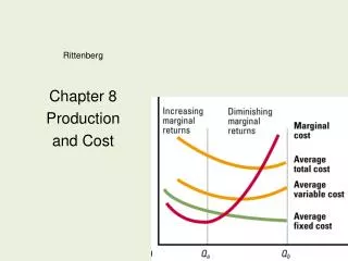
Marginal Costs • Marginal cost (MC): the change in cost caused by a change in output. • When marginal cost is greater than average cost, average cost rises -- ATC curve slopes up. • When marginal cost is below ATC, then ATC falls -- ATC curve slopes down.
Definition of Costs • Total Costs (TC) -- the expenses a business has in supplying goods and/or services. • Total Fixed Costs (TFC) -- payments to resources whose quantities can not be changed during a fixed period of time – the short run. (= total costs when Q=0) • Total Variable Costs (TVC) -- payments for additional resources used as output increases. (=total costs – total fixed costs) • These costs are relevant, but their curves will not be as important to us as the next page.
Definition of Costs • Average Fixed Cost -- the total fixed cost divided by total output. (= total fixed costs/quantity) • Average total Cost (SRATC): -- the total cost of production divided by the total quantity of output produced when at least one resource is fixed (= total costs/quantity) • Average Variable Cost -- total variable cost divided by total output ( = total variable cost/quantity) • Marginal Cost -- Additional cost associated with producing one more unit ( = Δ Total Costs = Δ Total Variable Costs)
Marginal-Average Rule The marginal cost curve intersects the minimum points of the average total cost and average variable cost curves
Short vs. Long Run • The short run refers to any period of time during which at least one resource can not be changed. • In the long run, everything is variable – nothing is fixed. • The most important difference between the short run and the long run is that the law of diminishing marginal returns does notapply when all resources are variable.
Economics of Scale • Scale means size. • Economies of scale: the decrease in per unit costs as the quantity of production increases and all resources are variable • Diseconomies of scale: the increase in per unit costs as the quantity of production increases and all resources are variable • Constant returns to scale: unit costs remain constant as the quantity of production is increased and all resources are variable
Economies of Scale and Long-Run Cost Curves • In the long run, a firm has many sizes to choose from. • The short run requires that scale be fixed— only one or a few resources can be changed.
Long- and Short-Run Average Cost Curves Each plant size can be represented by a U-shaped short-run average total cost curve. The firm’s long-run average cost curve is the “envelope” of these and other possible short-run average total cost curves • it is a smooth curve drawn so that it just touches the short-run curves without intersecting any of them.
Long-Run Average Total Cost • Long-run average total cost (LRATC):the smooth curve drawn so that it just touches the short-run curves without intersecting any of them. • The long-run average total cost curve gets its shape from economies and diseconomies of scale. • NOT from diminishing marginal returns
Shape of LRATC • If producing each unit of output becomes less costly there are economies of scale. • If producing each unit of output becomes more costly there are diseconomies of scale. • If unit costs remain constant as output rises there are constant returns to scale.
Long-Run and Short-Run Cost Curves (2) In some unusual cases Economies of Scale may prevail over the entire range of an industry’s realistic market scale. In this case, one very large firm would be the natural outcome and the most efficient use of resources.
Long-Run and Short-Run Cost Curves (3) In some rare cases scale may not be relevant at all. Firms of various sizes could compete with each other without any cost advantage from economies of scale.
Minimum Efficient Scale • Most industries experience both economies and diseconomies of scale. • The minimum efficient scale (MES)is the minimum point of the long-run average-cost curve; the output level at which the cost per unit of output is the lowest. • The MES varies considerably across industries.