Download
1 / 112
1.13k likes | 1.33k Views
NEUTRINO OSCILLATIONS Luigi DiLella Marienburg Castle August 2002. Content of these lectures :. Short introduction to neutrinos Formalism of neutrino oscillations in vacuum Solar neutrinos: Production Results Formalism of neutrino oscillations in matter

E N D
NEUTRINO OSCILLATIONS Luigi DiLella Marienburg Castle August 2002 Content of these lectures: • Short introduction to neutrinos • Formalism of neutrino oscillations in vacuum • Solar neutrinos: • Production • Results • Formalism of neutrino oscillations in matter • Future experiments • Atmospheric neutrinos • LSND and KARMEN experiments • Oscillation searches at accelerators: • Long baselineexperiments • Short baseline experiments • Long-term future • Conclusions
Neutrinos in the Standard Model Measurement of the Z width at LEP: only three light neutrinos (ne, nm, nt) Neutrino mass mn = 0 “by hand” two-component neutrinos: helicity (spin component parallel to momentum) = – 1 for neutrinos + 1 for antineutrinos p spin p spin n: n: helicity +1 neutrinos helicity –1 antineutrinos do not exist If mn > 0 helicity is not a good quantum number (helicity has opposite sign in a reference frame moving faster than the neutrino) massive neutrinos and antineutrinos can exist in both helicity states Are neutrinos Dirac or Majorana particles? Dirac neutrinos: n n lepton number is conserved Examples: neutron decay N P + e– + ne pion decay p+m+ + nm Majorana neutrinos: n n (only one four-component spinor field) lepton number is NOT conserved
Neutrinoless double–b decay: a way (the only way?) to distinguish Dirac from Majorana neutrinos (A, Z) (A, Z+2) + e– + e– violates lepton number conservation can only occur for Majorana neutrinos A second-order weak process: Process needs neutrino helicity flip between emission and absorption (neutron decay emits positive helicity neutrinos, neutrino capture by neutrons requires negative helicity) neutrinolessdouble–b decay can only occur if m(ne) > 0 Transition Matrix Element m(ne) The most sensitive search for double-b decay: 76Ge32 76Se34 + e– + e– E (e–1) + E (e–2) = 2038 keV p e– p e– n n ne two neutrons of the same nucleus Heidelberg–Moscow experiment: Five enriched76Ge crystals (solid–state detectors) Total mass: 19.96 kg , 86% 76Ge (natural Germanium contains only 7.7% 76Ge) Crystals are surrounded by anticoincidence counters and installed in underground Gran Sasso National Laboratory (Italy) Search for mono–energetic line at 2038 keV No evidence for neutrinoless double-b decay: m(ne) < 0.2 eV for Majorana neutrinos
Neutrino mass: relevance to cosmology A prediction of Big Bang cosmology: the Universe is filled with a Fermi gas of neutrinos at temperature T 1.9 K. Density ~60 n cm–3 , 60 n cm–3 for each neutrino type (ne, nm, nt) Critical density of the Universe : H0: Hubble constant (Universe present expansion rate) H0 = 100 h0 km s–1 Mpc –1(0.6 < h0 <0.8) GN: Newton constant Neutrino energy density (normalized to rc): Wn = 1 for Recent evidence from the study of distant Super-Novae: rc consists of ~30% matter (visible or invisible) and ~70% “vacuum energy” Cosmological models prefer non-relativistic dark matter (easier galaxy formation) with rn 20% of matter density cosmological limit on neutrino masses Direct measurements of neutrino masses ne: mc2 < 2.5 eV(from precise measurements of the electron energy spectrum from 3H decay) nm: mc2 < 0.16 MeV (from a precise measurement of m+ momentum from p+ decay at rest) nt: mc2 < 18.2 MeV(from measurements of t nt + 3, 5 or 6 p at LEP) With the exception of ne direct measurements of neutrino masses have no sensitivity to reach the cosmologically interesting region
Neutrino interaction with matter W–boson exchange: Charged–Current (CC) interactions Quasi-elastic scattering ne + n e– + p ne + p e+ + n nm + n m– + p nm + p m+ + n Energythreshold: ~112 MeV nt + n t – + p nt + p t+ + n Energythreshold: ~3.46 GeV Cross-section for energies >> threshold: sQE 0.45 x 10–38 cm2 Deep-inelastic scattering (DIS) (scattering on quarks, e.g. nm + d m– + u) ne + N e– + hadrons ne + N e+ + hadrons (N: nucleon) nm + N m– + hadrons nm + N m+ + hadrons nt + N t – + hadrons nt + N t+ + hadrons Cross-sections for energies >> threshold: sDIS(n) 0.68E x 10–38 cm2(E in GeV) sDIS( n ) 0.5sDIS(n) Z–boson exchange: Neutral–Current (NC) interactions Flavour-independent: the same for all three neutrino types n + N n + hadrons n + N n + hadrons Cross-sections: sNC( n) 0.3sCC(n) sNC( n ) 0.37sCC( n) Very low cross-sections: mean free path of a 10 GeV nm 1.7x10¹³ g cm–2 equivalent to 2.2x10⁷ km of Iron
0.8 0.6 0.4 0.2 0.0 sCC(nt) sCC(nm) Suppression of t production by nt CC interactions from t mass effects Neutrino – electron scattering 0 20 40 60 80 100 n Z e nee – W e–ne E (n) [GeV] Cross-section: s = A x10–42E cm2 (E in GeV) ne: A 9.5ne : A 3.4 nm, nt: A 1.6nm, nt : A 1.3 (all three n types) (ne only) Note: cross-section on electrons is much smaller than cross-section on nucleons because s GF2 W2 (W total energy in the centre-of-mass system) and W2 2meEn
NEUTRINO OSCILLATIONS The most promising way to verify if mn > 0 (Pontecorvo 1958; Maki, Nakagawa, Sakata 1962) Basic assumption: neutrino mixing e, , are not mass eigenstates but linear superpositions of mass eigenstates 1, 2, 3 with masses m1, m2, m3, respectively: • = e, , (“flavour” index) i = 1, 2, 3 (mass index) Uai: unitary mixing matrix
Time evolution of a neutrino state of momentum p created as at time t=0 Note: are different if mj mk phases appearance of neutrino flavour at t > 0 Case of two-neutrino mixing mixing angle For at production (t = 0):
Probability to detect at time t if pure was produced at t = 0 Natural units: m2 m22 – m12 (in vacuum!) Note: for m << p Use more familiar units: L = ct distance between neutrino source and detector Units:Dm2 [eV2]; L [km]; E [GeV] (or L [m]; E [MeV]) NOTE: Pab depends on Dm2 and not on m. However, if m1 << m2 (as for charged leptons and quarks), then Dm2m22m12 m22
Define oscillation length l: Units:l [km]; E [GeV]; Dm2 [eV2] (or l [m]; E [MeV]) Larger E, smaller Dm2 Smaller E, larger Dm2 sin2(2) Distance from neutrino source
Disappearance experiments Use a beam of na and measure na flux at distance L from source Measure Examples: • Oscillation experiments using ne from nuclear reactors (En few MeV: under threshold for m or t production) • nm detection at accelerators or from cosmic rays (to search for nmnt oscillations if En is under threshold for t production) Main uncertainty: knowledge of the neutrino flux for no oscillation the use of two detectors (if possible) helps n beam Far detector measures Paa Near detector measures n flux n source
Appearance experiments Use a beam of na and detect nb (b a)at distance L from source • Examples: • Detect ne + Nucleon e- + hadrons in a nm beam • Detect nt + Nucleon t - + hadrons in a nm beam (Energy threshold 3.5 GeV) NOTES • nbcontamination in beam must be precisely known (ne/nm 1% in nm beams from high-energy accelerators) • Most neutrino sources are not mono-energetic but have wide energy spectra. Oscillation probabilities must be averaged over neutrino energy spectrum.
Under the assumption of two-neutrino mixing: • Observation of an oscillation signal allowed region Dm2 versus sin2(2) • Negative result upper limit to Pab (Pab< P) exclusion region Large Dm2 short l Average over source and detector size: Small Dm2 long l: log(Dm2) (the start of the first oscillation) 0 1 sin2(2)
PARAMETERS OF OSCILLATION SEARCH EXPERIMENTS Neutrino source Flavour Baseline L Energy Minimum Dm2 Sun ne1.5 x 108 km 0.2 15 MeV 10-11 eV2 nmne nm ne 10 km 13000 km 0.2 GeV 100 GeV Cosmic rays 10-4 eV2 20 m 250 km Nuclear reactors ne <E> 3 MeV 10-1 10-6 eV2 nmne nm ne 15 m 730 km 20 MeV 100 GeV Accelerators 10-3 10 eV2 EVIDENCE/HINTS FOR NEUTRINO OSCILLATIONS • Solar Neutrino Deficit: ne disappearance between Sun and Earth • Atmospheric neutrino problem: deficit of nm coming from the other side of the Earth • LSND Experiment at Los Alamos: excess of ne in a beam consisting mainly of nm ,ne and nm
SOLAR NEUTRINOS Birth of a visible star: gravitational contraction of a cloud of primordial gas (mostly 75% H2, 25% He) increase of density and temperature in the core ignition of nuclear fusion Balance between gravity and pressure hydrostatic equilibrium Final result from a chain of fusion reactions: 4p He4 + 2e+ + 2ne Average energy produced in the form of electromagnetic radiation: Q = (4Mp– MHe4 + 2me)c2 – <E(2ne)> 26.1 MeV (<E(2ne)> 0.59 MeV) (from 2e+ + 2e– 4g) Sun luminosity: L = 3.846x1026 W = 2.401x1039 MeV/s Neutrino emission rate: dN(ne)/dt = 2 L/Q 1.84x1038 s –1 Neutrino flux on Earth: F(ne) 6.4x1010 cm–2 s –1 (average Sun-Earth distance = 1.496x10¹¹ m)
STANDARD SOLAR MODEL (SSM) (developed and continuously updated by J.N. Bahcall since 1960) Assumptions: • hydrostatic equilibrium • energy production by fusion • thermal equilibrium (energy production rate = luminosity) • energy transport inside the Sun by radiation Input: • cross-sections for fusion processes • opacity versus distance from Sun centre Method: • choose initial parameters • evolution to present time (t = 4.6x10⁹ years) • compare measured and predicted properties • modify initial parameters (if needed) Present Sun properties: Luminosity L = 3.846x1026 W RadiusR = 6.96x10⁸ m Mass M = 1.989x1030 kg Core temperature Tc = 15.6x10⁶ K Surface temperature Ts = 5773 K Hydrogen fraction in core = 34.1% (initially 71%) Helium fraction in core = 63.9% (initially 27.1%) as measured on surface today
Two fusion reaction cycles pp cycle (98.5% of L) p + p e+ + ne + d p + p e+ + ne + d or (0.4%): p + e– + p ne + d p + d g + He3 p + d g + He3 He3 +He3 He4 + p + p or (2x10⁻⁵): He3 + p He4 + e+ + ne 85% p + p e+ + ne + d p + d g + He3 He3 +He4 g + Be7 p + Be7 g + B8 e– + Be7 ne + Li7 B8 Be8 + e+ + ne p + Li7 He4 +He4 Be8 He4 +He4 15% or (0.13%) CNO cycle (two branches) p + N15 C12 +He4 p + N15 g+O16 p + C12 g+N13 p + O16 g+F17 N13 C13 + e+ + ne F17 O17 + e+ + ne p + C13 g+N14 p + O17 N14 +He4 p + N14 g+O15 O15 N15 + e+ + ne NOTE #1: in all cycles 4p He4 + 2e+ + 2ne NOTE #2: present solar luminosity originates from fusion reactions which occurred ~ 106 years ago. However, the Sun is practically stable over ~ 108 years.
Expected neutrino fluxes on Earth (pp cycle) Notations pp : p + p e+ + ne + d 7Be : e– + Be7 ne + Li7 pep : p + e– + p ne + d 8B : B8 Be8 + e+ + ne hep : He3 + p He4 + e+ + ne Line spectra: cm-2 s-1 Continuous spectra: cm-2 s-1 MeV -1 Radial distributions of neutrino production inside the Sun, as predicted by the SSM
The Homestake experiment (1970–1998): first detection of solar neutrinos A radiochemical experiment (R. Davis, University of Pennsylvania) ne + Cl 37 e– + Ar 37 Energy threshold E(ne) > 0.814 MeV Detector: 390 m3C2Cl4 (perchloroethylene) in a tank installed in the Homestake gold mine (South Dakota, U.S.A.) under 4100 m water equivalent (m w.e.) (fraction of Cl 37 in natural Chlorine = 24%) Expected production rate of Ar 37 atoms 1.5 per day Experimental method: every few months extract Ar 37 by N2 flow through tank, purify, mix with natural Argon, fill a small proportional counter, detect radioactive decay of Ar 37: e– + Ar 37 ne + Cl 37(half-life t1/2 = 34 d) (Final state excited Cl 37 atom emits Augier electrons and/or X-rays) Check efficiencies by injecting known quantities of Ar 37 into tank Results over more than 20 years of data taking SNU (Solar Neutrino Units): the unit to measure event rates in radiochemical experiments: 1 SNU = 1 event s–1 per 1036 target atoms Average of all measurements: R(Cl 37) = 2.56 0.16 0.16 SNU (stat) (syst) SSM prediction: 7.6 SNU Solar Neutrino Deficit +1.3 –1.1
Real-time experiments using water Čerenkov counters to detect solar neutrinos Neutrino – electron elastic scattering:n + e– n + e– Detect Čerenkov light emitted by recoil electron in water (detection threshold ~5 MeV) Cross-sections: s(ne) 6 s(nm) 6 s(nt) (5MeV electron path in water 2 cm) W and Z exchange Only Z exchange Two experiments: Kamiokande (1987 – 94). Useful volume: 680 m3 Super-Kamiokande (1996 – 2001). Useful volume: 22500 m3 installed in the Kamioka mine (Japan) at a depth of 2670 m w.e. Verify solar origin of neutrino signal from angular correlation between recoil electron and incident neutrino directions cosqsun
Super-Kamiokande detector Cylinder, height=41.4 m, diam.=39.3 m 50 000 tons of pure water Outer volume (veto) ~2.7 m thick Inner volume: ~ 32000 tons (fiducial mass 22500 tons) 11200 photomultipliers, diam.= 50 cm Light collection efficiency ~40% Inner volume while filling
Recoil electron kinetic energy distribution from ne– e elastic scattering of mono-energetic neutrinos is almost flat between 0 and 2En/(2 + me/En) convolute with predicted spectrum to obtain SSM prediction for electron energy distribution En SSM prediction Events/day Data 6 8 10 12 14 Electron kinetic energy (MeV) Results from 22400 events (1496 days of data taking) Measured neutrino flux (assuming all ne): F(ne) = (2.35 0.02 0.08) x 106 cm-2 s –1 (stat) (syst) SSM prediction: F(ne) = (5.05 ) x 106 cm-2 s –1 Data/SSM = 0.465 0.005 (stat) +1.01 –0.81 +0.093 –0.074 ne DEFICIT (including theoretical error)
Comparison of Homestake and Kamioka results with SSM predictions 0.465 0.016 2.56 0.23 Homestake and Kamioka results were known since the late 1980’s. However, the solar neutrino deficit was not taken seriously at that time. Why?
The two main solar ne sources in the Homestake and water experiments: He3 +He4 g + Be7 e– + Be7 ne + Li7 (Homestake) p + Be7 g + B8 B8 Be8 + e+ + ne (Homestake, Kamiokande, Super-K) Fusion reactions strongly suppressed by Coulomb repulsion Ec Z1Z2e2/d R2 R1 d Potential energy: Z1e Z2e d ~R1+R2 (R1 + R2 in fm) Ec 1.4 MeV for Z1Z2 = 4, R1+R2 = 4 fm Average thermal energy in the Sun core <E> = 1.5 kBTc 0.002 MeV (Tc=15.6 MK) kB (Boltzmann constant) = 8.6 x 10⁻⁵ eV/deg.K Nuclear fusion in the Sun core occurs by tunnel effect and depends strongly on Tc
Nuclear fusion cross-section at very low energies Nuclear physics term difficult to calculate measured at energies ~0.1– 0.5 MeV and assumed to be energy independent Tunnel effect: v = relative velocity Predicted dependence of the ne fluxes on Tc: From e– + Be7 ne + Li7: F(ne) Tc8 From B8 Be8 + e+ + ne : F(ne) Tc18 F TcN DF/F = N DTc/Tc How precisely do we know the temperature T of the Sun core? Search for ne from p + p e+ + ne + d (the main component of the solar neutrino spectrum, constrained by the Sun luminosity) very little theoretical uncertainties
Gallium experiments: radiochemical experiments to search for • ne + Ga71 e– + Ge71 • Energy threshold E(ne) > 0.233 MeV reaction sensitive to solar neutrinos • from p + p e+ + ne + d (the dominant component) • Three experiments: • GALLEX (Gallium Experiment, 1991 – 1997) • GNO (Gallium Neutrino Observatory, 1998 – ) • SAGE (Soviet-American Gallium Experiment) In the Gran Sasso National Lab 150 km east of Rome Depth 3740 m w.e. In the Baksan Lab (Russia) under the Caucasus. Depth 4640 m w.e. • Target: 30.3 tons of Gallium in HCl solution (GALLEX, GNO) • 50 tons of metallic Gallium (liquid at 40°C) (SAGE) • Experimental method: every few weeks extract Ge71 in the form of GeCl4 (a highly volatile • substance), convert chemically to gas GeH4, inject gas into a proportional counter, detect • radioactive decay of Ge71: e– + Ge71 ne + Ga71 (half-life t1/2 = 11.43 d) • (Final state excited Ga71 atom emits X-rays: detect K and L atomic transitions) • Check of detection efficiency: • Introduce a known quantity of As71 in the tank (decaying to Ge71: e– + Ge71 ne + Ga71) • Install an intense radioactive source producing mono-energetic ne near the tank: e– + Cr51 ne + V51 (prepared in a nuclear reactor, initial activity 1.5 MCurie equivalent to 5 times the solar neutrino flux),E(ne) = 0.750 MeV, half-life t1/2 = 28 d
Ge71 production rate ~1 atom/day +6.5 –6.1 SAGE (1990 – 2001) 70.8 SNU SSM PREDICTION: 128 SNU Data/SSM = 0.56 0.05 +9 –7
0.4650.016 Data are consistent with: • Full ne flux from p + p e+ + ne + d • ~50% of the ne flux from B8 Be8 + e+ + ne • Very strong (almost complete) suppression of the ne flux from e– + Be7 ne + Li7 The real solar neutrino puzzle: There is evidence for B8 in the Sun (with deficit 50%), but no evidence for Be7; yet Be7 is needed to make B8 by the fusion reaction p + Be7 g + B8 Possible solutions: • At least one experiment is wrong • The SSM is totally wrong • The ne from e– + Be7 ne + Li7are no longer ne when they reach the Earth and become invisible ne OSCILLATIONS
Unambiguous demonstration of solar neutrino oscillations: SNO (the Sudbury Neutrino Observatory in Sudbury, Ontario, Canada) SNO: a real-time experiment detecting Čerenkov light emitted in1000 tons of high purity heavy water D2O contained in a 12 m diam. acrylic sphere, surrounded by 7800 tons of high purity water H2O Light collection: 9456 photomultiplier tubes, diam. 20 cm, on a spherical surface with a radius of 9.5 m Depth: 2070 m (6010 m w.e.) in a nickel mine Electron energy detection threshold: 5 MeV Fiducial volume: reconstructed event vertex within 550 cm from the centre
Solar neutrino detection at SNO: • (ES) Neutrino – electron elastic scattering: n + e– n + e– Directional,s(ne) 6 s(nm) 6 s(nt) (as in Super-K) (CC) ne + d e–+ p + p Weakly directional: recoil electron angular distribution 1 – (1/3) cos(qsun) Good measurement of the ne energy spectrum (because the electron takes most of the ne energy) (NC) n + dn + p + n Equal cross-sections for all three neutrino types Measure the total solar flux from B8 Be8 + e+ + nin the presence of oscillations by comparing the rates of CC and NC events Detection of n + dn + p + n Detect photons ( e+e–) from neutron capture at thermal energies: • First phase (November 1999 – May 2001): n + d H3 + g (Eg = 6.25 MeV) • Second phase (in progress): add high purity NaCl (2 tons) n + Cl 35Cl 36 + g – ray cascade (S Eg 8. 6 MeV) • At a later stage: insert He3 proportional counters in the detector n + He3p + H3 (mono-energetic signal)
SNO expectations • Use three variables: • Signal amplitude (MeV) • cos(qsun) • Event distance from centre (R) (measured from the PM relative times) (R/Rav)3 (proportional to volume) cos(qsun) (Rav = 6 m = radius of the acrylic sphere) Use b and g radioactive sources to calibrate the energy scale Use Cf252 neutron source to measure neutron detection efficiency (14%) Neutron signal does not depend on cos(qsun)
From 306.4 days of data taking: Number of events with kinetic energy Teff > 5 MeV and R < 550 cm: 2928 Neutron background: 78 12 events. Background electrons 45 events +18 –12 Use likelihood method and the expected distributions to extract the three signals
Solar neutrino fluxes, as measured separately from the three signals: FCC(ne) = 1.76 x 106 cm-2s-1 FES(n) = 2.39 x 106 cm-2s-1 FNC(n) = 5.09 x 106 cm-2s-1 +0.06 +0.09 –0.05 –0.09 Note: FCC(ne) F(ne) Calculated under the assumption that all incident neutrinos are ne +0.24 +0.12 –0.23 –0.12 FSSM(n) = 5.05 x 106 cm-2s-1 +0.44 +0.46 –0.43 –0.43 +1.01 –0.81 stat. syst. stat. and syst. errors combined FNC(n) – FCC(ne) = F(nmt) = 3.33 0.64 x 106 cm–2 s –1 5.2 standard deviations from zero evidence that solar neutrino flux on Earth contains sizeable nm or nt component (in any combination) Write FES(n) as a function of F(ne) andF(nmt): (because ) F(n) = F(ne) + F(nmt)
Interpretation of the solar neutrino data using the two-neutrino mixing hypothesis Vacuum oscillations ne spectrum on Earth F(ne) = Pee F0(ne) (F0(ne)spectrum at production) ne disappearance probability L = 1.496 x 10¹¹ m (average Sun – Earth distance with 3.3% yearly variation from eccentricity of Earth orbit) Fit predicted ne spectrum to data using q, Dm2 as adjustable parameters L [m] E [MeV] Dm2 [eV2] 4x10⁻¹⁰ eV2 10–10 4x10–11 Regions of oscillation parameters consistent with solar neutrino data available before the end of the year 2000
NEUTRINO OSCILLATIONS IN MATTER (L. Wolfenstein, 1978) Neutrinos propagating through matter undergo refraction. p: neutrino momentum N: density of scattering centres f(0): forward scattering amplitude (at = 0°) Refraction index: In vacuum: Plane wave in matter: = ei(np•r –Et) (for e << 1) But energy must be conserved! Add a term V neutrino potential energy in matter V < 0: attractive potential (n > 1) V > 0: repulsive potential (n < 1)
Neutrino potential energy in matter 1. Contribution from Z exchange (the same for all three flavours) n n Z GF: Fermi coupling constant Np (Nn): proton (neutron) density w: weak mixing angle e,p,n e,p,n 2. Contribution from W exchange (only for ne!) ne e- W+ matter density [g/cm3] electron density e- ne NOTE: V(n) = – V( n )
Example: two-neutrino mixing between ne and nm in a constant density medium(same results for mixing between ne and nt) Use flavour basis: Evolution equation: 2x2 matrix (Remember: for M p) NOTE: m1, m2, are defined in vacuum
Rewrite: diagonal term: no mixing term responsible for ne–nm mixing r = constant time-independent H Diagonalize non-diagonal term in H to obtain mass eigenvalues and eigenstates Eigenvalues in matter [eV2] (r in g/cm3, E in MeV) Mixing angle in matter For x = Dm2cos2qxres mixing becomes maximal (qm = 45°) even if the mixing angle in vacuum is very small: “MSW resonance” (discovered by Mikheyev and Smirnov in 1985) Notes: MSW resonance can exist only if q < 45° (otherwise cos2q < 0) For nex < 0 no MSW resonance if q < 45°
M2 M22 M12 Mass eigenvalues versus x Oscillation length in matter: (l oscillation length in vacuum) At x = xres:
Matter-enhanced solar neutrino oscillations Solar neutrinos are produced in a high-density medium (the Sun core) and travel through variable density r = r(t) Use formalism of neutrino oscillations in matter: Evolution equationHn= i n / t H (2 x 2 matrix) depends on time t through r(t) H has no eigenstates Solve the evolution equation numerically: solar density vs. radius 100 10 1 0.1 r [g/cm3] R/RO 0. 0.2 0.4 0.6 0.8 (pure ne at production) (d = very small time interval) (until neutrino escapes from the Sun)
It is always possible to write: (|a1|2 + |a2|2 = 1) where n1, n2 are the “local” eigenstates of the time-independent Hamiltonian for fixed r At production (t=0, in the Sun core): [;n1(0), n2(0) eigenstates of H for r=r(0)] Assume q (mixing angle in vacuum) < 45°: cosq > sinq in vacuum qm> 45° at production if x > xres : x > xres (Dm2 in eV2, r in g/cm3) A simple class of solutions ( “adiabatic solutions”): a1a1(0), a2a2 (0) at all t (if r varies slowly over an oscillation length) At exit from the Sun (t=tE): M2 n1(tE), n2(tE) :mass eigenstates in vacuum In vacuum (because q < 45° in vacuum) qm < 45° qm > 45° ne DEFICIT
Regions of the (Dm2 , sin22q) plane allowed by the solar neutrino flux measurements in the Homestake, Super-K and Gallium experiments Different energy thresholds different regions of the (Dm2 , sin22q) plane Super-K The regions common to the three measurements contain the allowed oscillation parameters
Matter-enhanced solar neutrino oscillations (“MSW solutions”) (using only data available before the end of the year 2000) Survival probability versus neutrino energy LMA SMA 10–5 eV 2 LOW sin22q 10–3 10–2 10–1 LMA: Large Mixing Angle SMA: Small Mixing Angle
Additional experimental information Energy spectrum distortions Super-K 2002 Data/SSM Electron kinetic energy (MeV) SNO recoil electron spectrum from ne + d e–+ p + p SNO data/SSM prediction ne deficit is energy independent within errors (no distortions)
Seasonal variation of measured neutrino flux in Super-K Yearly variation of the Sun-Earth distance: 3.3% seasonal variation of the solar neutrino flux for some vacuum oscillation solutions Note: expected seasonal variation from change of solid angle 6.6% Days since start of data taking The observed effect is consistent with the variation of solid angle alone
Day-night effects (expected for some MSW solutions from matter-enhanced oscillations when neutrinos traverse the Earth at night increase of ne flux at night) Subdivide night spectrum into bins of Sun zenith angle to study dependence on path length inside Earth and density cos(Sun zenith angle) SNO Day and Night Energy Spectra (CC + ES + NC events) Difference Night – Day
SK data: comparison with oscillations Sun zenith angle distributions for different electron energy bins Electron energy distribution Vacuum oscillation SMA LMA LOW • Vacuum oscillation and SMA solution disagree with electron energy distribution • LMA and LOW solutions describe reasonably well the zenith angle distributions • No dependence on zenith angle within errors
Global fits to all existing solar neutrino data 48 data points, two free parameters (mixing angle q, Dm2) 46 degrees of freedom LMA solution: 2 = 43.5; Dm2 = 6.9x10– 5 eV2; q = 31.7° (BEST FIT) LOW solution: 2 = 52.5; Dm2 = 7.2x10– 8 eV2; q = 39.1° D2 = 9; Prob(D2 9) = 1.1% (marginally acceptable) LMA Dm2 [eV2] The present interpretation of all solar neutrino data using two-neutrino mixing Note: variable tan2q is preferred to sin22q because sin22q is symmetric around q = 45° and MSW solutions are possible only if q < 45° tan2q
Verification of the LMA solution using antineutrinos from nuclear reactors Nuclear reactors: intense, isotropic sources of ne from b decay of neutron-rich fission fragments ne production rate: 1.9x10²⁰ Pths–1(Pth [GW]: reactor thermal power) Broad energy spectrum extending to 10 MeV, <E> 3 MeV Uncertainty on the expected ne flux: ±2.7 % Detection: ne+ p e+ + n(on the free protons of hydrogen – rich liquid scintillator) thermalization by multiple collisions (<t> 180 ms), followed by capture e+ e– 2gn + p d +g (Eg = 2.2 MeV) prompt signal delayed signal E = En – 0.77 MeV KAMioka Liquid scintillator Anti-Neutrino Detector (KAMLAND) ne source: several nuclear reactors surrounding the Kamioka site Total power 70 GW — average distance 175 35 km (long baseline) Expected ne flux (no oscillations) 1.3 x 106 cm–2 s–1 ~550 events/year Average oscillation length <losc> 110 km for Dm2 = 6.9 x 10⁻⁵eV 2 (LMA) expect large ne deficit with measurable energy modulation
KAMLAND detector 1000 tons liquid scintillator Transparent balloon Mineral oil Acrylic sphere Photomultipliers (1879) (coverage: 35% of 4p) Outer detector (pure H2O) 225 photomultipliers 13 m 18 m