Download
1 / 96
1.03k likes | 1.33k Views
Explore econometric models for binary, multinomial, count data, and censored variables in car ownership analysis based on income. Understand odds ratios and interpret coefficients in regression.

E N D
Econometrics 2 - Lecture 2Models with Limited Dependent Variables
Contents • Limited Dependent Variable Cases • Binary Choice Models • Binary Choice Models: Estimation • Binary Choice Models: Goodness of Fit • Application to Latent Models • Multi-response Models • Multinomial Models • Count Data Models • The Tobit Model • The Tobit Model: Estimation • The Tobit II Model Hackl, Econometrics 2, Lecture 2
Example Explain whether a household owns a car: explanatory power have • income • household size • etc. Regression for describing car-ownership is not suitable! • Owning a car has two manifestations: yes/no • Indicator for owning a car is a binary variable Models are needed that allow to describe a binary dependent variable or a, more generally, limited dependent variable Hackl, Econometrics 2, Lecture 2
Cases of Limited Dependent Variables Typical situations: functions of explanatory variables are used to describe or explain • Dichotomous or binary dependent variable, e.g., ownership of a car (yes/no), employment status (employed/unemployed), etc. • Ordered response, e.g., qualitative assessment (good/average/bad), working status (full-time/part-time/not working), etc. • Multinomial response, e.g., trading destinations (Europe/Asia/Africa), transportation means (train/bus/car), etc. • Count data, e.g., number of orders a company receives in a week, number of patents granted to a company in a year • Censored data, e.g., expenditures for durable goods, duration of study with drop outs Hackl, Econometrics 2, Lecture 2
Example: Car Ownership and Income What is the probability that a randomly chosen household owns a car? • Sample of N=32 households, among them 19 households with car • Proportion of car owning households:19/32 = 0.59 • Estimated probability for owning a car: 0.59 • But: The probability will differ for rich and poor! • The sample data contain income information: • Yearly income: average EUR 20.524, minimum EUR 12.000, maximum EUR 32.517 • Proportion of car owning households among the 16 households with less than EUR 20.000 income: 9/16 = 0.56 • Proportion of car owning households among the 16 households with more than EUR 20.000 income: 10/16 = 0.63 Hackl, Econometrics 2, Lecture 2
Car Ownership and Income, cont’d How can a model for the probability – or prediction – of car ownership take the income of a household into account? Notation: N households • dummy yi for car ownership; yi =1: household i has car • income of i-th household: xi2 For predicting yi – or estimating the probability P{yi =1} – , a model is needed that takes the income into account Hackl, Econometrics 2, Lecture 2
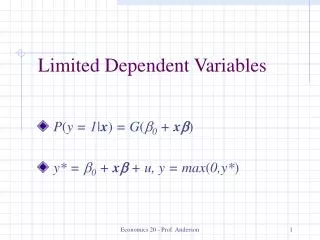
Modelling Car Ownership How is car ownership related to the income of a household? • Linear regression yi = xi’β + εi = β1+ β2xi2 + εi • With E{εi|xi} = 0, the model yi = xi’β + εi gives P{yi =1|xi} = xi’β due to E{yi|xi} = 1*P{yi =1|xi} + 0*P{yi =0|xi} = P{yi =1|xi} • The systematic part of yi = xi’β + εi, xi’β, is P{yi =1|xi}! • Model for y is specifying the probability for y = 1as a function of x • Problems: • xi’β not necessarily in [0,1] • Error terms: for a given xi • εi can take on only two values, viz. 1- xi’β and xi’β • V{εi|xi} = xi’β(1- xi’β), heteroskedastic, dependent upon β Hackl, Econometrics 2, Lecture 2
Modelling Car Ownership, cont’d • Use of a function G(xi,β) with values in the interval [0,1] P{yi =1|xi} = E{yi|xi} = G(xi,β) • Standard logistic distribution function L(z) fulfils limz→ -∞ L(z) = 0, limz→ ∞ L(z) = 1 • Binary choice model: P{yi =1|xi} = pi = L(xi’β) = [1 + exp{-xi’β}]-1 • Can be written using the odds ratio pi/(1- pi) for the event {yi =1|xi} • Interpretation of coefficients β: An increase of xi2 by 1 results in a relative change of the odds ratio pi/(1- pi) by β2 or by 100β2%; cf. the notion semi-elasticity Hackl, Econometrics 2, Lecture 2
Car Ownership and Income, cont’d E.g., P{yi =1|xi} = 1/(1+exp(-zi)) with z = -0.5 + 1.1*x, the income x in EUR 1000 per month • Increasing income is associated with an increasing probability of owning a car: z goes up by 1.1 for every additional EUR 1000 • For a person with an income of EUR 1000, z = 0.6 and the probability of owning a car is 1/(1+exp(-0.6)) = 0.646 Standard logistic distribution function L(z), with z on the horizontal and L(z) on the vertical axis Hackl, Econometrics 2, Lecture 2
Odds, Odds Ratio The odds or the odds ratio (in favour) of event A is the ratio of the probability that A will happen to the probability that A will not happen • If the probability of success is 0.8 (that of failure is 0.2), the odds of success are 0.8/0.2 = 4; we say, “the odds of success are 4 to 1” • If the probability of event A is p, that of “not A” therefore being 1-p, the odds or the odds ratio of event A is the ratio p/(1-p) • We say the odds (ratio) of A is “p/(1-p) to 1” or “1 to (1-p)/p” • The logarithm of the odds p/(1-p) is called the logit of p Hackl, Econometrics 2, Lecture 2
Betting Odds • The probability of success is 0.8 • The odds of success are 4 to 1 • Betting odds for success are 1:4 • The bookmaker is prepared to pay out a prize of one fourth of the stake and return the stake as well, to anyone who places a bet on success Hackl, Econometrics 2, Lecture 2
Contents • Limited Dependent Variable Cases • Binary Choice Models • Binary Choice Models: Estimation • Binary Choice Models: Goodness of Fit • Application to Latent Models • Multi-response Models • Multinomial Models • Count Data Models • The Tobit Model • The Tobit Model: Estimation • The Tobit II Model Hackl, Econometrics 2, Lecture 2
Binary Choice Models Model for probability P{yi =1|xi}, function of K (numerical or categori-cal) explanatory variables xi and unknown parameters β, such as E{yi|xi} = P{yi =1|xi} = G(xi,β) Typical functions G(xi,β): distribution functions (cdf’s) F(xi’β) = F(z) • Probit model: standard normal distribution function; V{z} = 1 • Logit model: standard logistic distribution function; V{z}=π2/3=1.812 • Linear probability model (LPM) Hackl, Econometrics 2, Lecture 2
Linear Probability Model (LPM) Assumes that P{yi =1|xi} = xi’β for 0 ≤ xi’β ≤ 1 but sets restrictions P{yi =1|xi} = 0 for xi’β < 0 P{yi =1|xi} = 1 for xi’β > 1 • Typically, the model is estimated by OLS, ignoring the probability restrictions • Standard errors should be adjusted using heteroskedasticity-consistent (White) standard errors Hackl, Econometrics 2, Lecture 2
Probit Model: Standardization E{yi|xi} = P{yi =1|xi} = F(xi’β): assume F(.) to be the distribution function of N(0, σ2) • Given xi, the ratio β/σ2 determines P{yi =1|xi} • Standardization restriction 2 = 1: allows unique estimates for β Hackl, Econometrics 2, Lecture 2
Probit vs Logit Model • Differences between the probit and the logit model: • Shapes of distribution are slightly different, particularly in the tails. • Scaling of the distributions is different: The implicit variance for i in the logit model is 2/3 = (1.81)2, while 1 for the probit model • Probit model is relatively easy to extend to multivariate cases using the multivariate normal or conditional normal distribution • In practice, the probit and logit model produce quite similar results • The scaling difference makes the values of not directly comparable across the two models, while the signs are typically the same • The estimates of in the logit model are roughly a factor /3 1.81 larger than those in the probit model Hackl, Econometrics 2, Lecture 2
Marginal Effects of Binary Choice Models Linear regression model E{yi|xi} = xi’β: the marginal effect E{yi|xi}/xikof a change in xkis βk For E{yi|xi} = F(xi’β) • The marginal effect of changing xk • Probit model: ϕ(xi’β) βk, with standard normal density function ϕ • Logit model: exp{xi’β}/[1 + exp{xi’β}]2 βk • Linear probability model: βk if xi’β is in [0,1] • In general, the marginal effect of changing the regressor xk depends upon xi’β, the shape of F, and βk; the sign is that of βk Hackl, Econometrics 2, Lecture 2
Interpretation of Binary Choice Models The effect of a change in xk can be characterized by the • “Slope”, i.e., the “average” marginal effect or the gradient of E{yi|xi} for the sample means of the regressors • For a dummy variable D: marginal effect is calculated as the difference of probabilities P{yi =1|x(d),D=1} – P{yi =1|x(d),D=0}; x(d) stands for the sample means of all regressors except D • For the logit model: The coefficient βk is the relative change of the odds ratio when increasing xk by 1 unit Hackl, Econometrics 2, Lecture 2
Contents • Limited Dependent Variable Cases • Binary Choice Models • Binary Choice Models: Estimation • Binary Choice Models: Goodness of Fit • Application to Latent Models • Multi-response Models • Multinomial Models • Count Data Models • The Tobit Model • The Tobit Model: Estimation • The Tobit II Model Hackl, Econometrics 2, Lecture 2
Binary Choice Models: Estimation Typically, binary choice models are estimated by maximum likelihood Likelihood function, given N observations (yi, xi) L(β) = Πi=1NP{yi =1|xi;β}yi P{yi =0|xi;β}1-yi = ΠiF(xi’β)yi (1- F(xi’β))1-yi • Maximization of the log-likelihood function ℓ(β) = log L(β) = Si yi log F(xi’β) + Si (1-yi) log (1-F(xi’β)) • First-order conditions of the maximization problem • ei: generalized residuals Hackl, Econometrics 2, Lecture 2
Generalized Residuals The first-order conditions Sieixi = 0 define the generalized residuals • The generalized residuals ei can assume two values, depending on the value of yi: • ei = f(xi’b)/F(xi’b) if yi =1 • ei = - f(xi’b)/(1-F(xi’b)) if yi =0 b are the estimates of β • Generalized residuals are orthogonal to each regressor; cf. the first-order conditions of OLS estimation Hackl, Econometrics 2, Lecture 2
Estimation of Logit Model • First-order condition of the maximization problem gives [due to P{yi =1|xi} = pi = L(xi,β)] • From Sixi = Siyixi follows – given that the model contains an intercept –: • The sum of estimated probabilities Si equals the observed frequency Siyi • Similar results for the probit model, due to similarity of logit and probit functions Hackl, Econometrics 2, Lecture 2
Binary Choice Models in GRETL Model > Nonlinear Models > Logit > Binary • Estimates the specified model using error terms with standard logistic distribution Model > Nonlinear Models > Probit > Binary • Estimates the specified model using error terms with standard normal distribution Hackl, Econometrics 2, Lecture 2
Example: Effect of Teaching Method Study by Spector & Mazzeo (1980); see Greene (2003), Chpt.21 Personalized System of Instruction: a new teaching method in economics; has it an effect on student performance in later courses? • Data: • GRADE (0/1): indicator whether grade was higher than in principal course • PSI (0/1): participation in program with new teaching method • GPA: grade point average • TUCE: score on a pre-test, entering knowledge • 32 observations Hackl, Econometrics 2, Lecture 2
Effect of Teaching Method, cont’d Logit model for GRADE, GRETL output Model 1: Logit, using observations 1-32 Dependent variable: GRADE Coefficient Std. Error z-stat Slope* const -13.0213 4.93132 -2.6405 GPA 2.82611 1.26294 2.2377 0.533859 TUCE 0.0951577 0.141554 0.6722 0.0179755 PSI 2.37869 1.06456 2.2344 0.456498 Mean dependent var 0.343750 S.D. dependent var 0.188902 McFadden R-squared 0.374038 Adjusted R-squared 0.179786 Log-likelihood -12.88963 Akaike criterion 33.77927 Schwarz criterion 39.64221 Hannan-Quinn 35.72267 *Number of cases 'correctly predicted' = 26 (81.3%) f(beta'x) at mean of independent vars = 0.189 Likelihood ratio test: Chi-square(3) = 15.4042 [0.0015] Predicted 0 1 Actual 0 18 3 1 3 8 Hackl, Econometrics 2, Lecture 2
Effect of Teaching Method, cont’d Estimated logit model for the indicator GRADE P{GRADE = 1} = p = L(z) = exp{z}/(1+exp{z}) with z = −13.02 + 2.826*GPA + 0.095*TUCE + 2.38*PSI = log {p/(1-p)} = logit{p} • Regressors • GPA: grade point average • TUCE: score on a pre-test, entering knowledge • PSI (0/1): participation in program with new teaching method • Slopes • GPA: 0.53 • TUCE: 0.02 • Difference P{GRADE =1|x(d),PSI=1} – P{GRADE =1|x(d), PSI=0}: 0.49; cf. Slope 0.46 Hackl, Econometrics 2, Lecture 2
Effect of Teaching Method, cont’d Logit model for GRADE, actual and fitted values of 32 observations Hackl, Econometrics 2, Lecture 2
Properties of ML Estimators • Consistent • Asymptotically efficient • Asymptotically normally distributed These properties require that the assumed distribution is correct • Correct shape • No autocorrelation and/or heteroskedasticity • No dependence – correlations – between errors and regressors • No omitted regressors Hackl, Econometrics 2, Lecture 2
Contents • Limited Dependent Variable Cases • Binary Choice Models • Binary Choice Models: Estimation • Binary Choice Models: Goodness of Fit • Application to Latent Models • Multi-response Models • Multinomial Models • Count Data Models • The Tobit Model • The Tobit Model: Estimation • The Tobit II Model Hackl, Econometrics 2, Lecture 2
Goodness-of-Fit Measures Concepts • Comparison of the maximum likelihood of the model with that of the naïve model, i.e., a model with only an intercept, no regressors • pseudo-r2 • McFadden R2 • Index based on proportion of correctly predicted observations or hit rates • Rp2 Hackl, Econometrics 2, Lecture 2
McFadden R2 Based on log-likelihood function • ℓ(b) = ℓ1: maximum log-likelihood of the model to be assessed • ℓ0: maximum log-likelihood of the naïve model, i.e., a model with only an intercept; ℓ0 ≤ ℓ1 and ℓ0, ℓ1 < 0 • The larger ℓ1 - ℓ0, the more contribute the regressors • ℓ1 = ℓ0,if all slope coefficients are zero • ℓ1 = 0, if yi is exactly predicted for all i • pseudo-r2: a number in [0,1), defined by • McFadden R2: a number in [0,1], defined by • Both are 0 if ℓ1 = ℓ0, i.e., all slope coefficients are zero • McFadden R2 attains the upper limit 1 if ℓ1 = 0 Hackl, Econometrics 2, Lecture 2
Naïve Model: Calculation of ℓ0 Maximum log-likelihood function of the naïve model, i.e., a model with only an intercept: ℓ0 • P{yi =1} = p for all i (cf. urn experiment) • Log-likelihood function log L(p) = N1 log(p) + (N – N1) log (1-p) with N1 = Siyi, i.e., the observed frequency • Maximum likelihood estimator for p is N1/N • Maximum log-likelihood of the naïve model ℓ0 = N1 log(N1/N) + (N – N1) log (1 – N1/N) Hackl, Econometrics 2, Lecture 2
Goodness-of-fit Measure Rp2 Comparison of correct and incorrect predictions • Predicted outcome ŷi = 1 if F(xi’b) > 0.5, i.e., if xi’b > 0 = 0 if F(xi’b) < 0.5, i.e., if xi’b ≤ 0 • Cross-tabulation of actual and predicted outcome • Proportion of incorrect predictions wr1 = (n01+n10)/N • Hit rate: 1 - wr1 proportion of correct predictions • Comparison with naive model: • Predicted outcome of naïve model ŷi = 1 for all i (!), if = N1/N> 0.5; ŷi = 0 for all iif ≤ 0.5 • wr0 = 1 - if > 0.5, wr0 = if ≤ 0.5 • Goodness-of-fit measure: Rp2= 1 – wr1/wr0; may be negative! Hackl, Econometrics 2, Lecture 2
Example: Effect of Teaching Method Study by Spector & Mazzeo (1980); see Greene (2003), Chpt.21 Personalized System of Instruction: new teaching method in economics; has it an effect on student performance in later courses? • Data: • GRADE (0/1): indicator whether grade was higher than in principal course • PSI (0/1): participation in program with new teaching method • GPA: grade point average • TUCE: score on a pre-test, entering knowledge • 32 observations Hackl, Econometrics 2, Lecture 2
Effect of Teaching Method, cont’d Logit model for GRADE, GRETL output Model 1: Logit, using observations 1-32 Dependent variable: GRADE Coefficient Std. Error z-stat Slope* const -13.0213 4.93132 -2.6405 GPA 2.82611 1.26294 2.2377 0.533859 TUCE 0.0951577 0.141554 0.6722 0.0179755 PSI 2.37869 1.06456 2.2344 0.456498 Mean dependent var 0.343750 S.D. dependent var 0.188902 McFadden R-squared 0.374038 Adjusted R-squared 0.179786 Log-likelihood -12.88963 Akaike criterion 33.77927 Schwarz criterion 39.64221 Hannan-Quinn 35.72267 *Number of cases 'correctly predicted' = 26 (81.3%) f(beta'x) at mean of independent vars = 0.189 Likelihood ratio test: Chi-square(3) = 15.4042 [0.0015] Predicted 0 1 Actual 0 18 3 1 3 8 Hackl, Econometrics 2, Lecture 2
Effect of Teaching Method, cont’d Logit model for GRADE, actual and fitted values of 32 observations Hackl, Econometrics 2, Lecture 2
Effect of Teaching Method, cont’d Comparison of the LPM, logit, and probit model for GRADE • Estimated models: coefficients and their standard errors • Coefficients of logit model: due to larger variance, larger by factor √(π2/3)=1.81 than that of the probit model • Very similar slopes Hackl, Econometrics 2, Lecture 2
Effect of Teaching Method, cont’d Goodness-of-fit measures for the logit model • With N1 = 11 and N = 32 ℓ0 = 11 log(11/32) + 21 log(21/32) = - 20.59 • As = N1/N = 0.34 < 0.5: the proportion wr0of incorrect predictions with the naïve model is wr0 = = 11/32 = 0.34 • From the GRETL output: ℓ1 = -12.89, wr1 = 6/32 Goodness-of-fit measures • McFadden R2 = 1 – (-12.89)/(-20.59) = 0.374 • pseudo-R2 = 1 - 1/[1 + 2(-12.89 + 20.59)/32) = 0.325 • Rp2 = 1 – wr1/wr0 = 1 – 6/11 = 0.45 Hackl, Econometrics 2, Lecture 2
Contents • Limited Dependent Variable Cases • Binary Choice Models • Binary Choice Models: Estimation • Binary Choice Models: Goodness of Fit • Application to Latent Models • Multi-response Models • Multinomial Models • Count Data Models • The Tobit Model • The Tobit Model: Estimation • The Tobit II Model Hackl, Econometrics 2, Lecture 2
Modelling Utility Latent variable yi*: utility difference between owning and not owning a car; unobservable (latent) • Decision on owning a car • yi* > 0: in favour of car owning • yi* ≤ 0: against car owning • yi* depends upon observed characteristics (e.g., income) and unobserved characteristics εi yi* = xi’β + εi • Observation yi = 1 (i.e., owning car) if yi* > 0 P{yi =1} = P{yi* > 0} = P{xi’β + εi > 0} = 1 – F(-xi’β) = F(xi’β) last step requires a distribution function F(.) with symmetric density Latent variable model: based on a latent variable that represents the underlying behaviour Hackl, Econometrics 2, Lecture 2
Latent Variable Model Model for the latent variable yi* yi* = xi’β + εi yi*: not necessarily a utility difference • εi‘s are independent of xi’s • εi has a standardized distribution • Probit model if εi has standard normal distribution • Logit model if εi has standard logistic distribution • Observations • yi = 1 if yi* > 0 • yi = 0 if yi* ≤ 0 • ML estimation Hackl, Econometrics 2, Lecture 2
Contents • Limited Dependent Variable Cases • Binary Choice Models • Binary Choice Models: Estimation • Binary Choice Models: Goodness of Fit • Application to Latent Models • Multi-response Models • Multinomial Models • Count Data Models • The Tobit Model • The Tobit Model: Estimation • The Tobit II Model Hackl, Econometrics 2, Lecture 2
Multi-response Models Models for explaining the choice between discrete outcomes • Examples: • Working status (full-time/part-time/not working), qualitative assessment (good/average/bad), etc. • Trading destinations (Europe/Asia/Africa), transportation means (train/bus/car), etc. • Multi-response models describe the probability of each of these outcomes, as a function of variables like • person-specific characteristics • alternative-specific characteristics • Types of multi-response models (cf. above examples) • Ordered response models: outcomes have a natural ordering • Multinomial (unordered) models: ordering of outcomes is arbitrary Hackl, Econometrics 2, Lecture 2
Example: Credit Rating Credit rating: numbers, indicating experts’ opinion about (a firm’s) capacity to satisfy financial obligations, e.g., credit-worthiness • Standard & Poor's rating scale: AAA, AA+, AA, AA-, A+, A, A-, BBB+, BBB, BBB-, BB+, BB, BB-, B+, B, B-, CCC+, CCC, CCC-, CC, C, D • Verbeek‘s data set CREDIT • Categories “1“, …,“7“ (highest) • Investment grade with alternatives “1” (better than category 3) and “0” (category 3 or less, also called “speculative grade“) • Explanatory variables, e.g., • Firm sales • Ebit, i.e., earnings before interest and taxes • Ratio of working capital to total assets Hackl, Econometrics 2, Lecture 2
Ordered Response Model Choice between M alternatives Observed alternative for sample unit i: yi • Latent variable model yi* = xi’β + εi with K-vector of explanatory variables xi yi = j if γj-1 < yi* ≤γj for j = 0,…,M • M+1 boundaries γj, j = 0,…,M, with γ0 = -∞, …, γM = ∞ • εi‘s are independent of xi’s • εi typically follows the • standard normal distribution: ordered probit model • standard logistic distribution: ordered logit model Hackl, Econometrics 2, Lecture 2
Example: Willingness to Work Married females are asked: „How much would you like to work?“ Potential answers of individual i: yi = 1 (not working), yi = 2 (part time), yi = 3 (full time) • Measure of the desired labour supply • Dependent upon factors like age, education level, husband‘s income Ordered response model with M = 3 yi* = xi’β + εi with yi = 1 if yi* ≤ 0 yi = 2 if 0 < yi* ≤ γ yi = 3 if yi* > γ • εi‘s with distribution function F(.) • yi* stands for “willingness to work” or “desired hours of work” Hackl, Econometrics 2, Lecture 2
Willingness to Work, cont’d In terms of observed quantities: P{yi = 1 |xi} = P{yi* ≤ 0 |xi} = F(-xi’β) P{yi = 3 |xi} = P{yi* > γ |xi} = 1 - F(γ -xi’β) P{yi = 2 |xi} = F(γ -xi’β) – F(-xi’β) • Unknown parameters: γ and β • Standardization: wrt location (γ = 0) and scale (V{εi} = 1) • ML estimation Interpretation of parameters β • Wrtyi*(= xi’β + εi): willingness to work increases with larger xk for positive βk • Wrt probabilities P{yi = j |xi}, e.g., for positive βk • P{yi = 3 |xi} = P{yi* > γ |xi}increases and • P{yi = 1 |xi} P{yi* ≤ 0 |xi}decreases with larger xk Hackl, Econometrics 2, Lecture 2
Example: Credit Rating Verbeek‘s data set CREDIT: 921 observations for US firms' credit ratings in 2005, including firm characteristics Rating models: • Ordered logit model for assignment of categories “1“, …,“7“ (highest) • Binary logit model for assignment of “investment grade” with alternatives “1” (better than category 3) and “0” (category 3 or less, also called “speculative grade“) Hackl, Econometrics 2, Lecture 2
Credit Rating, cont’d Verbeek‘s data set CREDIT Ratings and characteristics for 921 firms: summary statistics _____________________ Book leverage: ratio of debts to assets Hackl, Econometrics 2, Lecture 2
Credit Rating, cont’d Verbeek, Table 7.5. Hackl, Econometrics 2, Lecture 2