Download
1 / 30
300 likes | 501 Views
Routing. Lesson 10 NETS2150/2850 http://www.ug.cs.usyd.edu.au/~nets2150/. School of Information Technologies. Lesson Outline. Know the characteristics of unicast routing protocol Understand various ways of routing Routing Strategies Experiment with common routing algorithms

E N D
Routing Lesson 10 NETS2150/2850 http://www.ug.cs.usyd.edu.au/~nets2150/ School of Information Technologies
Lesson Outline • Know the characteristics of unicast routing protocol • Understand various ways of routing • Routing Strategies • Experiment with common routing algorithms • Dijsktra’s Algorithm of OSPF • Bellman-Ford Algorithm of RIP
Graph abstraction for routing algorithms: graph nodes are routers graph edges are physical links link cost/weight: delay, $ cost or congestion level A D E B F C Routing protocol Routing Goal: find “good” path thru network from source to destination. • “good” path: • typically means minimum cost path
Routing protocol establish mutually consistent routing tables in every router Characteristics of routing protocol: Correctness Simplicity Robustness Stability Fairness Optimality Efficiency application transport network data link physical application transport network data link physical Routing in Packet Switched Network network data link physical 1. Send data 2. Receive data Packet switching network
Performance Criteria • How to select “best” path? • Used for selection of path • Minimum hop • Least cost IP routing table Destination Gateway Netmask Iface 129.78.8.0 0.0.0.0 255.255.252.0 eth0 127.0.0.0 0.0.0.0 255.0.0.0 lo 0.0.0.0 129.78.11.254 0.0.0.0 eth0
Example Packet Switched Network Link cost • Shortest path VS • Least-cost path
Routing Strategies • Fixed • Flooding • Random • Adaptive
Fixed Routing • Single permanent path for each source to destination pair • Path fixed, at least until a change in network topology
Fixed RoutingTables Network Topology
Flooding • Packet sent by node to every neighbour and the neighbour sends to its neighbours • Incoming packets retransmitted on every link except incoming link • Eventually a number of copies will arrive at destination • Each packet is uniquely numbered so duplicates can be discarded • To bound the flood, max hop count is included in the packets If (Packet’s hop count = = max_hop_count) discard!
Properties of Flooding • All possible routes are tried • Very robust • At least one packet will have taken minimum hop count or “best” route • All nodes are visited • The common approach used to distribute routing information, like a node’s link costs to neighbours
Random Routing • Node selects one outgoing path for retransmission of incoming packet • Selection can be random or round robin • Can select outgoing path based on probability calculation • Path is typically not “best” one • Used in ‘hot potato routing’ • nodes have no buffer to store packets • packets routed to any path of the lowest delay
Adaptive Routing • Used by almost all packet switching networks • Routing decisions change as conditions on the network change • Failure • Congestion • Requires info about network • Decisions more complex
Adaptive Routing - Advantages • Improved performance • Aids congestion control by exercising load balancing across different alternative paths • But, it is complex • Reacting too quickly can cause oscillation • Too slowly, may not be relevant
Routing Algorithm classification Global or decentralised information? Global: • all routers have complete topology, link cost info • Known as “link state” algorithms • E.g. Dijkstra’s Algorithm Decentralised: • router knows physically-connected neighbours, i.e link costs to neighbours • iterative process of computation, exchange of info with neighbours • Known as “distance vector” algorithms • E.g. Bellman-Ford Algorithm
Routing Algorithms • Given network of nodes connected by bi-directional links • Each link has a cost in each direction and may be different • Cost of path between two nodes is sum of costs of links traversed • For each pair of nodes, find a path with the least cost
Dijkstra’s Algorithm Definitions • Find shortest paths from given source node to all other nodes, by developing paths in order of increasing path length • N= set of nodes in the network • s = source node • T= set of nodes so far incorporated by the algorithm • w(i, j)= link cost from node i to node j • w(i, i) = 0 • w(i, j) = if the two nodes are not directly connected • w(i, j) 0 if the two nodes are directly connected • L(n)=cost of least-cost path from node s to node n
Dijkstra’s Algorithm • Step 1 [Initialization] • T = {s} Set of nodes so far incorporated consists of only source node • L(n) = w(s, n) for n ≠ s • Step 2[Get Next Node] • Find neighbouring node, x, not in T with least-cost path from s • Incorporate node x into T • Step 3[Update Least-Cost Paths] • L(n) = min[L(n), L(x) + w(x, n)]for all nÏ T • Algorithm terminates when all nodes have been added to T
Dijkstra’s Algorithm Notes • At termination, value L(x) associated with each node x is cost of least-cost path from s to x. • One iteration of steps 2 and 3 adds one new node to T • Defines least cost path from s to that node
5 5 3 3 5 2 5 2 2 2 2 2 3 3 1 1 2 2 2 2 T = {A} T = {A,D} 5 5 3 3 5 2 5 2 2 2 2 2 3 3 1 1 A A A A A A D D D D D D B E B E B E E B E E B B F F F F F F C C C C C C 2 2 2 2 T = {A,D,B} T = {A,D,B,E} 5 5 3 3 5 5 2 2 2 2 2 2 3 3 1 1 2 2 2 2 T = {A,D,B,E,C} T = {A,D,B,E,C,F}
Bellman-Ford Algorithm Definitions • Find shortest paths from given node considering at most one hop away • Then, find the shortest paths with a constraint of paths of at most two hops. Then 3 hops, and so on… • s = source node • w(i, j)=link cost from node i to node j • w(i, i) = 0 • w(i, j) = if the two nodes are not directly connected • w(i, j) 0 if the two nodes are directly connected • h = maximum number of hops (links) in path • Lh(n)=cost of least-cost path from s to n, at most h hops away
Bellman-Ford Algorithm • Step 1 [Initialization] • Lh(s) = 0, for all h • L0(n) = , for n s • Step 2 [Update] • For each successive h > 0 and each node n: • If Lh(n) > minj[Lh(j) + w(j,n)] Then • Lh+1(n)=minj[Lh(j)+w(j,n)] • Connect n with predecessor node j that achieves minimum cost
5 5 3 3 5 2 5 2 2 2 2 2 3 3 1 1 2 2 2 2 h = 1 h = 2 5 5 3 3 A A A A D D D D B E B E B E B E F F F F C C C C 5 2 5 2 2 2 2 2 3 3 1 1 2 2 2 2 h = 3 h = 4
Algorithms Comparison • Results from two algorithms agree • Information gathered • Bellman-Ford • Each node can maintain set of costs and paths for every other node • Only exchange information with direct neighbours • Can update costs and paths based on information from neighbours and knowledge of link costs • Used as part of the Routing Information Protocol (RIP) • Dijkstra • Each node needs complete topology • Must know link costs of all links in network • Must exchange information with all other nodes • Used as part of Open Shortest Path First Protocol (OSPF)
Physical Spec: 533 MHz VIA C3 processor 128 MB SDRAM Runs on Linux Three onboard 10/100 Ethernet ports 1 or 2 T1/E1 ports Software spec: PPP, Cisco HDLC & frame relay ATM PPPoE & PPPoA Routing procotols: RIP, RIP II, OSPF, IS-IS & BGP4 Example: ImageStream’s TransPort™ router
Summary • Routing is the process of finding a path from a source to every destination in the network • Different routing strategies available • Common adaptive routing: • Dijsktra’s algorithm • Bellman-Ford algorithm • Read Stallings Section 12.2 and 12.3 • Next: Functions of internetwork layer protocol