introduction to statistics
mortuza ahmmed

introduction to statistics
E N D
Presentation Transcript
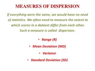
MEASURES OF DISPERSION If everything were the same, we would have no need of statistics. We often need to measure the extent to which scores in a dataset differ from each other. Such a measure is called dispersion. • Range (R) • Mean Deviation (MD) • Variance • Standard Deviation (SD)
Range The range is the difference between the highest and lowest values of a dataset. For the dataset {4, 6, 9, 3, 7} the lowestvalue is 3, highest is 9 so the range is 9-3=6.
Mean Deviation It is the mean of the absolute deviations of a set of data about the mean. For sample size N, It is defined by
Why Coefficient of Variation The coefficient of variation (CV) is used to compare different sets of data having different of measurement. The wages of workers may be in dollars and the consumption of meat in their families may be in kilograms. The standard deviation of wages in dollars cannot be compared with the standard deviation of amounts of meat in kilograms. Both the standard deviations need to be converted into coefficient of variation for comparison. Suppose the value of CV for wages is 10% and the value of CV for kilograms of meat is 25%. This means that the wages of workers are consistent.
Example A company has 2 sections with 40 and 65 employees .Their average weekly wages are $450 and $350. The SDs are 7 and 9. (i) Which section has a larger wage bill? (ii) Which section has larger variability in wages? Wage bill for section A = 40 x 450 = 18000Wage bill for section B = 65 x 350 = 22750Section B is larger in wage bill. CV for Section A = 7/450 x 100 =1.56 % CV for Section B = 9/350 x 100 = 2.57% There is greater variability in the wages of section B.
Correlation It is a statistical technique that can show whether and how strongly pairs of variables are related. The average weight of people 5'5'' is less than the average weight of people 5'6'', and their average weight is less than that of people 5'7'', etc. Correlation can tell us just how much of the variation in peoples' weights is related to their heights.
Positive correlation As the values of a variable increase, the values of the other variable also increase. As the values of a variable decrease, the values of the other also decrease. Relation between price and supply
Negative correlation As the values of a variable increase, the values of the other variable decrease. As the values of a variable decrease, the values of the other variable increase. Relation between price and demand
Zero correlation Here, change in one variable has no effect on the other variable. Relation between height and exam grades
Interpretation of correlation coefficient • r = 0 indicates no relation • r = + 1 indicates a perfect positive relation • r = - 1 indicates a perfect negative relation • Values of r between 0 and 0.3 (0 and - 0.3) indicate a weak positive (negative) relation • Values of r between .3 and .7 (- .3 and - .7) indicate a moderate positive (negative) relation • Values of r between 0.7 and 1 (- 0.7 and -1) indicate a strong positive (negative) relation
Interpretation a gives expected amount of change in Y for X=0 b gives expected amount of change in Y for 1 unit change in X
Example 5 cards are chosen at random from a deck of 52 playing cards. What is the probability of choosing 5 aces? P (5 aces) = 0 / 52 = 0
Experiment An action where the result is uncertain is called an experiment. Tossing a coin
Sample Space All possible outcomes of an experiment is called sample space. A die is rolled, the sample space : S = {1, 2, 3, 4, 5, 6}
Event A single result of an experiment is called an event. Getting a Tail when tossing a coin
Example A die is rolled, find the probability that an even number is obtained. Sample Space , S = {1, 2, 3, 4, 5, 6} The event "an even number is obtained" E = {2, 4, 6} P (E) = n (E) / n(S) = 3 / 6
Example A teacher chooses a student at random from a class of 30 girls. What is the probability that the student chosen is a girl? P (girl) = 30 / 30 = 1
Example In a lottery, there are 10 prizes and 25 blanks. A lottery is drawn at random. Find the probability of getting a prize? P (getting a prize) = 10 / ( 10 + 25 ) = 10 / 35
Example At a car park there are 60 cars, 30 vans and 10 Lorries. If every vehicle is equally likely to leave, find the probability of: a)Van leaving first b) Lorry leaving first. • Let S be the sample space and A be the event of a van leaving first. So, n (S) = 100 , n (A) = 30 : P ( A ) = 30 / 100 b) Let B be the event of a lorry leaving first. So, n (S) = 100 , n (B) = 10, : P ( B ) = 10 / 100
Example In a box, there are 8 black, 7 blue and 6 green balls. One ball is picked up randomly. Find the probability that ball is neither black nor green? Total number of balls = (8 + 7 + 6) = 21 Let E= event that the ball drawn is neither black nor green = event that the ball drawn is blue. P ( E ) = 7 / 21
Example Two coins are tossed, find the probability that two heads are obtained. Each coin has 2 possible outcomes: H (heads)and T (Tails) Sample space, S = {(H, T), (H, H), (T, H), (T, T)} The event "two heads are obtained", E = {(H, H)} P (E) = 1 / 4
Example Two dice are rolled; find the probability that the sum of the values is equal to 1. The sample space, S = { (1,1),(1,2),(1,3),(1,4),(1,5),(1,6) (2,1),(2,2),(2,3),(2,4),(2,5),(2,6) (3,1),(3,2),(3,3),(3,4),(3,5),(3,6) (4,1),(4,2),(4,3),(4,4),(4,5),(4,6) (5,1),(5,2),(5,3),(5,4),(5,5),(5,6) (6,1),(6,2),(6,3),(6,4),(6,5),(6,6) } Let E be the event "sum equal to 1". P (E) = 0 / 36 = 0