EE/Ae 157 a Passive Microwave Sensing
510 likes | 674 Views
EE/Ae 157 a Passive Microwave Sensing. TOPICS TO BE COVERED. Rayleigh-Jeans Approximation Power-Temperature Correspondence Microwave Radiometry Models Bare Surfaces Vegetation Covered Surfaces Radiometer Implementations Total Power Radiometers Dicke Radiometers Applications

EE/Ae 157 a Passive Microwave Sensing
E N D
Presentation Transcript
TOPICS TO BE COVERED • Rayleigh-Jeans Approximation • Power-Temperature Correspondence • Microwave Radiometry Models • Bare Surfaces • Vegetation Covered Surfaces • Radiometer Implementations • Total Power Radiometers • Dicke Radiometers • Applications • Polar Ice Mapping • Soil Moisture Mapping
Thermal Radiation Laws • Heat energy is a special case of EM radiation • The random motion (due to collisions) of the molecules due to kinetic energy results in exitation (electronic, vibrational and rotational) followed by random emissions during decay • This leads to radiation over a large bandwidth according to Planck’s law for an ideal source (called a black body) • Thermal emission is usually unpolarized
Rayleigh-Jeans Approximation • When we can approximate the exponential term in Planck’s law by the first two terms in its Taylor series expansion, • Substituting this into Planck’s formula, we find • This approximation shows less than 1% deviation from Planck’s law as long as
Relationship between Surface Brightness and Spectral Radiant Emittance • The surface spectral radiant emittance is the integral over all angles of a quantity known as the surface brightness • If the brightness is independent of q, (a Lambertian surface) • The surface brightness is therefore given by
ANTENNA GROUND ELEMENT Power-Temperature Correspondence • The power per unit bandwidth radiated into a solid angle by a surface element with emissivity is • The antenna receives the energy with different amounts of gain from different angles. If the normalized gain pattern is the received power over a narrow bandwidth would be
ANTENNA GROUND ELEMENT ANTENNA GROUND ELEMENT Power-Temperature Correspondence • If the antenna has a receiving area , the solid angle subtended by the antenna is • Therefore, the received power is • The receiver integrates the energy received by the antenna from all angles. The solid angle subtended by the surface element when viewed from the antenna is
ANTENNA GROUND ELEMENT ANTENNA GROUND ELEMENT Power-Temperature Correspondence • Therefore, we can write the received power as • To find the total power received by the radiometer, we now have to integrate over the antenna angles and the bandwidth: • If this becomes
Power-Temperature Correspondence • The received power is usually written as • where the equivalent temperature is given by • The effective temperature observed by the radiometer is therefore the physical temperature of the surface, multiplied by a factor that is a function of the surface emissivity and the antenna pattern.
Microwave Radiometry ModelsBare Surface • In practice, the radiometer receive power not only from the surface radiation, but also from energy radiated by the sky and reflected by the surface
Microwave Radiometry ModelsBare Surface • The total power radiated by the surface is therefore • Following the same derivation as before, we find the equivalent temperature to be • Therefore, the equivalent microwave temperature is
Microwave Radiometry ModelsBare Surface • Since • we can rewrite the microwave temperature as • Note that the refection coefficient is a function of polarization, we will measure different microwave temperatures for different polarizations
Microwave Radiometry Models Reflection Coefficient • From Maxwell’s equations, one finds that
3 4 2 1 Microwave Radiometry Models Vegetation Cover
D D h h Radiometer Measurements: Circular Antenna Beam Side-Looking View Nadir View
Flight Path Nadir Line Scan Direction Conical Scan Geometry
10 5 Angle from Nadir 0 -5 -10 -5 5 -10 0 10 Angle from Nadir
Radiometer Implementations • The function of a radiometer is to measure the equivalent temperature of the scene, based on the amount of power delivered by the antenna to the receiver • The measurement process is characterized by two important attributes • accuracy • precision • The accuracy of the measurement depends on how well the radiometer is calibrated • The precision of the measurement defines the smallest change in temperature that the radiometer can measure reliably, and is driven by radiometer stability
Radiometer ImplementationsCalibration • To calibrate the transfer function of a radiometer, the output voltage is measured as a function of noise temperature of a source connected to the input terminals of the receiver
Radiometer ImplementationsTotal Power Radiometer • The output power is
Radiometer ImplementationsTotal Power Radiometer • Since the input power consists of thermal noise, the instantaneous voltage at the output of the IF amplifier has a Gaussian distribution with zero mean. • The output of the square law detector has an exponential distribution. Such a distribution has a standard deviation that is equal to its mean value. • Th output of the square law detector will therefore be a signal with a mean value, and a fluctuating part that has a standard deviation equal to the mean • It is this fluctuating part that limits the precision of the radiometer, and will be interpreted as random fluctuations in the measured system temperature
Radiometer ImplementationsTotal Power Radiometer • The effect of the low-pass filter is to smooth out the fluctuations in time. If the filter has an equivalent integration time the fluctuations at the output of the filter will have a standard deviation that is reduced by a factor • Therefore, at the output of the low-pass filter, we have • From an observational point of view, is the smallest change in temperature that the radiometer can measure reliably:
Radiometer ImplementationsEffect of System Gain Variations • Th previous analysis assumes the system to be perfect. Changes in receiver gain will also cause the output power to fluctuate. This will be interpreted as a temperature fluctuation equal to • Since the noise fluctuations, and the gain fluctuations are uncorrelated, the resulting uncertainty in the system temperature is • In many cases, the gain variations are the largest error source
Radiometer ImplementationsDicke Radiometer • Experimental results show that the bulk of the gain fluctuations are at frequencies lower than 1 Hz • A Dicke radiometer uses modulation techniques to reduce the effects of system gain variations • A Dicke radiometer is basically a total power radiometer with two additional features • A switch connexted to the receiver input (as close to the antenna as possible) that modulates the input signal • A synchronous demodulator placed between the square law detector and the low-pass filter • The modulation consists of periodically switching the receiver input between the antenna and a constant (reference) noise source
Radiometer ImplementationsDicke Radiometer • The switching rate is chosen so that over a period of one switching cycle is essentially constant, and therefore identical for the half cycle during which the receiver is connected to the antenna and the half cycle during which the receiver is connected to the reference source • The output of the square law detector is • Superimposed on these average values are fluctuations due to noise and gain fluctuations
Radiometer ImplementationsDicke Radiometer • The synchronized demodulator is consists of a switch operated synchronously with the input Dicke switch, followed by parallel amplifiers with opposite polarity • The output of these amplifiers are summed and fed to the low-pass filter • The output of the low-pass filter is • Which can be written as • Note that the output is independent of the receiver noise temperature
Radiometer ImplementationsDicke Radiometer • The fluctuating part of the radiometer output consists of three parts: • Gain variations that lead to an uncertainty • Noise variations, which after integrating over half the cycle lead to an uncertainty of • Noise on the second half of the integration cycle equal to
Radiometer ImplementationsDicke Radiometer • Assuming the uncertainties to be statistically independent, the total uncertainty is • This can be written as • This is known as the sensitivity of an unbalanced Dicke radiometer
Radiometer ImplementationsBalanced Dicke Radiometer • Of particular importance is the case where • This is a balanced Dicke radiometer • The sensitivity of the balanced Dicke radiometer becomes • The factor of 2 comes from the fact that the antenna is observed for only half the time • Several different approaches are used for balancing Dicke radiometers. The simplest (conceptually) involves using a feedback loop to control the reference temperature