Download

1 / 41
420 likes | 639 Views
Regression Commands in R. April 2nd, 2014 Computing for Research I. A S imple Experiment. What is the linear relationship between age and height?. ε. Y. ε. X. Linear Regression. For linear regression, R uses 2 functions. Could use function “ lm ”

E N D
Regression Commands in R April 2nd, 2014 Computing for Research I
A Simple Experiment What is the linear relationship between age and height?
ε Y ε X
Linear Regression • For linear regression, R uses 2 functions. • Could use function “lm” • Could use the generalized linear model (GLM) framework • function called “glm”
LM Function • lm(formula, data, subset, weights, na.action, method = "qr", model = TRUE, x = FALSE, y = FALSE, qr = TRUE, singular.ok = TRUE, contrasts = NULL, offset, ...) • reg1 <- lm(height~age, data=dat) #simple regression • reg2 <- lm(height ~ 1 , data=dat) #intercept only • http://stat.ethz.ch/R-manual/R-patched/library/stats/html/lm.html
LM Function • Can accommodate weights (weighted regression) • Survey weights, inverse probability weighting, etc. • Results including beta, SE(beta), Wald T-tests, p-values • Can obtain ANOVA, ANCOVA results • Can specify contrasts for predictors • Can do some regression diagnostics, residual analysis • Let’s have fun!
LM Example age <- c(18,19,20,21,22,23,24,25,26,27,28,29) height <- c(76.1,77,78.1,78.2,78.8,79.7,79.9,81.1,81.2,81.8,81.8,83.5) dat <- as.data.frame(cbind(age,height)) dat dim(dat) is.data.frame(dat) reg1 <- lm(height~age, data=dat) summary(reg1)
Summary(lm) • Call: lm function • Quantiles of Residuals • Coefficients • Residual standard error • R-squared • F-statistic
We have got linear regression done!Really???But it is not beer time yet!
4 Assumptions of linear regression • Linearity of Y in X • Independence of the residuals (error terms are uncorrelated) • Normality of residual distribution • Homoscedasticity of errors (constant variance)
Basic Checks par(mfrow=c(2,2)) par(mar=c(5,5,2,2)) attach(reg1) hist(residuals) plot(age,residuals) plot(fitted.values,residuals) plot(height,fitted.values) abline(0,1) • http://stat.ethz.ch/R-manual/R-patched/library/stats/html/plot.lm.html
Checks for homogeneity of error variance (1), normality of residuals (2), • and outliers respectively (3&4). • plot(reg1) #built in diagnostics
ANOVA X<-c(0,1,0,0,1,1,0,0,0) Y<-c(15,2,7,5,2,5,7,8,4) reg2 <- lm(Y~X) reg2.anova<-anova(reg2) names(reg2.anova) reg2.anova • Calculate R2 = Coefficient of determination • “Proportion of variance in Y explained by X” • R2 = 1- (SSerr/Sstot) R2 <- 1-(81.33/(43.56+81.33)) fstat<- reg2.anova$F pval <- reg2.anova$P
Generalized Linear Models • GLM contains: • A probability distribution from the exponential family • A linear predictor X • A link function g • We use the command:glm(formula, family = gaussian, data, weights, subset, na.action, start = NULL, etastart, mustart, offset, control = list(...), model = TRUE, method = "glm.fit", x = FALSE, y = TRUE, contrasts = NULL, ...) • GLMs default is linear regression, no need to specify link function or distribution. http://web.njit.edu/all_topics/Prog_Lang_Docs/html/library/base/html/glm.html
Generalized Linear Models • GLM takes the argument “family” • family = description of the error distribution and link function to be used in the model. This can be a character string naming a family function, a family function or the result of a call to a family function.
Some families family(object, ...) • binomial(link = "logit") • gaussian(link = "identity") #REGRESSION, DEFAULT • gamma(link = "inverse") • inverse.gaussian(link = "1/mu^2") • poisson(link = "log") • quasi(link = "identity", variance = "constant") • quasibinomial(link = "logit") • quasipoisson(link = "log")
Let’s look an example • Data From psychiatric study • X=number of daily hassles, predictor • Y=anxiety symptom, response • Do number of self reported hassles predict anxiety symptoms?
Code setwd("C:\\Users\\smartbenben\\Desktop") data1 <- read.table("data.dat", header = TRUE) hist(data1$HASSLES) plot(data1$HASSLES,data1$ANX) glm(ANX ~HASSLES, data = as.data.frame(data1)) #LINEAR REGRESSION IS DEFAULT. IF IT WERE NOT, WE'D #SPECIFY FAMILY glm.linear <- glm(ANX ~HASSLES, data = as.data.frame(data1), family = gaussian)
R output for GLM call glm(ANX ~HASSLES, data = as.data.frame(data1)) Call: glm(formula = ANX ~ HASSLES, data = as.data.frame(data1)) Coefficients: (Intercept) HASSLES 5.4226 0.2526 Degrees of Freedom: 39 Total (i.e. Null); 38 Residual Null Deviance: 4627 Residual Deviance: 2159 AIC: 279
Summary summary(glm.linear) #Gives more information Call: glm(formula = ANX ~ HASSLES, family = gaussian, data = as.data.frame(data1)) Deviance Residuals: Min 1Q Median 3Q Max -13.3153 -5.0549 -0.3794 4.5765 17.5913 Coefficients: Estimate Std. Error t value Pr(>|t|) (Intercept) 5.42265 2.46541 2.199 0.034 * HASSLES 0.25259 0.03832 6.592 8.81e-08 *** --- Signif. codes: 0 ‘***’ 0.001 ‘**’ 0.01 ‘*’ 0.05 ‘.’ 0.1 ‘ ’ 1 (Dispersion parameter for gaussian family taken to be 56.80561) Null deviance: 4627.1 on 39 degrees of freedom Residual deviance: 2158.6 on 38 degrees of freedom AIC: 279.05
How to Report Model Results • Beta coefficients (size, directionality) • Wald T tests and p-values • Potentially log likelihood or AIC values if doing model comparison names(glm.linear) #Many important things can be pulled off from a glm object that will be of use in coding your own software.
Intercept only model glm(ANX ~ 1, data = as.data.frame(data1)) Call: glm(formula = ANX ~ 1, data = as.data.frame(data1)) Coefficients: (Intercept) 19.65 Degrees of Freedom: 39 Total (i.e. Null); 39 Residual Null Deviance: 4627 Residual Deviance: 4627 AIC: 307.5
GLM summary(glm.linear) #Shows t-tests, pvals, etc ## code our own t-test ! #give the var-cov matrix of parameters var<-vcov(glm.linear) var beta <- glm.linear$coefficients[[2]] var.beta <- var[2,2] se.beta<-sqrt(var.beta) t.test <- beta/se.beta #SAME AS IN SUMMARY df<-glm.linear$df.residual
GLM # Results Table: results.table <- summary(glm.linear)$coefficients # compare to glm.linear$coefficients # pvalue for Wald test of slope: results.table[2,4] #LRTs. > glm.linear$null.deviance [1] 4627.1 > glm.linear$deviance [1] 2158.613
Plots for model check hist(glm.linear$residuals) plot(glm.linear$fitted.values,glm.linear$residuals)
Multiple regression – Anxiety data • Lets add gender to anxiety for previous model and refit glm. • 1=male, 0=female gender<- c(0,0,1,1,0,1,1,1,0,1,1,1,0,0,0,0,1,0,1,1,0,1,1,0,0,0,1,1,0,0,1,0,1,1,0,0,0,1,1,0) ANX <- data1$ANX HASSLES<-data1$HASSLES glm.linear2 <- glm(ANX ~HASSLES+gender)
Check assumptions • Spend some time to interpret the relevant output. par(mfrow=c(2,1)) hist(glm.linear2$residuals) plot(glm.linear2$fitted.values, glm.linear2$residuals)
Back to Regression Diagnostics • If you are analyzing a dataset carefully, you may consider regression diagnostics before reporting results • Typically, you look for outliers, residual normality, homogeneity of error variance, etc. • There are many different criteria for these things that we won’t review in detail. • Recall Cook’s Distance, Leverage Points, Dfbetas, etc. • CAR package from CRAN contains advanced diagnostics using some of these tests.
Multicollinearity • Two or more predictor variables in a multiple regression model are highly correlated • The coefficient estimates may change erratically in response to small changes in the model or the data • Indicators that multicollinearity: 1) Large changes in the estimated regression coefficients when a predictor variable is added or deleted 2) Insignificant regression coefficients for the affected variables in the multiple regression, but a rejection of the joint hypothesis that those coefficients are all zero (using an F-test)
Multicollinearity • A formal measure of multicollinearityis variance inflation factor (VIF) • VIF >10 indicates multicollinearity.
Regression diagnostics using LMCAR package #Fit a multiple linear regression on the MTCARS datalibrary(car) fit <- lm(mpg~disp+hp+wt+drat, data=mtcars) # Assessing Outliers outlierTest(fit) # Bonferonni p-value for most extreme obs qqPlot(fit, main="QQ Plot") #qq plot for studentizedresid leveragePlots(fit, ask=FALSE) # leverage plots # Influential Observations# Cook's D plot# identify D values > 4/(n-p-1) cutoff <- 4/((nrow(mtcars)-length(fit$coefficients)-2)) plot(fit, which=4, cook.levels=cutoff)
CAR for Diagnostics, normality # Distribution of studentized residualslibrary(MASS) sresid <- studres(fit) hist(sresid, freq=FALSE, main="Distribution of Studentized Residuals") #Overlays the normal distribution based on the observed studentized #residualsxfit<-seq(min(sresid),max(sresid),length=40) yfit<-dnorm(xfit) #Generate normal density based on observed resids lines(xfit, yfit)
CAR for Diagnostics, constant variance #Non-constant Error Variance # Evaluate homoscedasticity# non-constant error variance Score test ncvTest(fit) # plot studentized residuals vs. fitted values spreadLevelPlot(fit) #Multi-collinearity # Evaluate Collinearity vif(fit) # variance inflation factor
Assuming our Y were counts glm.poisson <- glm(ANX ~HASSLES, data=as.data.frame(data1), family = poisson) glm.poisson2 <- glm(ANX ~HASSLES, data =as.data.frame(data1), family = quasipoisson) summary(glm.poisson) summary(glm.poisson2) #Compare variance estimates Review: Poisson Regression What is overdispersion? What is Poisson parameter interpretation? What is overdispersed Poisson parameter interpretation?
Overdispersion in counts • Example: • Y= #red blood cell units administered, X=drug (aprotinin vs. lysine analogue) • Overdispersion • Excess 0: > 50% zeros
ZIP Model • Two component mixture model: model of structural zeros that do not originate from any process, and counts that originate from a Poisson process. • Thus, the 0/1 process is modeled separately from the Poisson process when the observed 0 is determined not to have arisen from a Poisson process • 0/1 binary process modeled as logistic regression • Count process simultaneously modeled as Poisson regression
VGAM Package library(VGAM) fit2 <- vglm(y ~ x1, zipoisson, trace = TRUE)
Results - ZIP • > summary(fit2) Call: vglm(formula = y ~ x1, family = zipoisson, trace = TRUE) Pearson Residuals: Min 1Q Median 3Q Max logit(phi) -1.8880 -0.93828 0.59499 0.86550 1.0504 log(lambda) -1.3104 -0.31901 -0.31901 -0.18509 10.3208 Coefficients: Value Std. Error t value (Intercept):1 -0.025409 0.16450 -0.15446 (Intercept):2 0.703619 0.08129 8.65569 x1:1 -0.040470 0.33087 -0.12231 x1:2 -0.774116 0.17667 -4.38181
Interpretation • Odds of observing a (structural) zero in blood product usage in the durg a versus drug l are exp(-.040) = 0.96[0.50,1.83]. • The risk of blood product usage in drug a versus drug l group is exp(-0.774) =0.46[0.33,0.65]. • Conclusion: there is a significant decreased risk of RBC usage in the aprotinin versus lysine analogue group.