Understanding Aggregate Planning: Strategies for Effective Production Management
Aggregate planning is a vital approach in production management, focusing on meeting demand throughout the year by developing a coherent production plan for a single representative product. This involves managing capacity, workforce, inventory, and outsourcing. By analyzing aggregate demand and aligning production output with fluctuations, organizations can balance short-term needs and long-term growth. This chapter covers planning levels, techniques, and strategies such as level capacity and chase demand to effectively manage resources and satisfy market demands.


Understanding Aggregate Planning: Strategies for Effective Production Management
E N D
Presentation Transcript
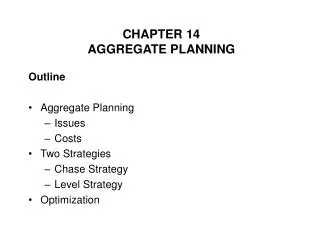
Chapter 12 Aggregate Plannig Ardavan Asef-Vaziri Systems and Operations Management
Aggregate Planning Long range Intermediate range Short range Now 2 months 1 Year Intermediate-range capacity planning Usually covers a period of 12 months.
Overview of Planning Levels • Long-range plans • Long term capacity • Location / layout • Intermediate plans (Aggregate Planning) • Manpower Utilization regular time, overtime • Outsourcing Buying from a third party • Inventorycarrying product for latter periods • Backlogsatisfying the demand of the earlier periods • Hiring and layoff • Short-range plans (Scheduling) • Job assignments • Machine loading
Aggregate Planning Aggregate planning is a big picture approach to production planning. It is a production plan to meet the demandthroughout the year. It is notconcerned with individual products, but with a single aggregate product representing all products. For example, in a TV manufacturing plant, the aggregate planning does not go into all models and sizes. It only deals with a single representative aggregate TV. Such an aggregate TV may even does not exist in reality. All models are lump together and represent a single product; hence the term aggregate planning.
Aggregate Planning Aggregate approach permits planners to develop intermediate-range capacity planning without being involved in too much details. In aggregate planning we are concerned with the quantity and also timing of demand. Demand is uneven through the year. Two basic characteristics of aggregate planning 1-Aggregate Product 2-Uneven Demand It begins with a forecast of aggregate demand for one year. Then a one year plan is prepared for each month. It includes volume of output, working hours, overtime, outsourcing, inventories, back orders, and hiring and layoffs.
Aggregate Planning 1-Demand 2-Regular time production 3-Overtime production 4-Outsourcing; buying from a third party 5-Inventory; production in one period and sale in one or more later periods. 6-Backlog; production in one period to satisfy the demand of one or more earlier periods. 7-Hiring and layoffs A number of aggregate plans are examined in terms of feasibility and their costs. The best one is selected.
Aggregate Planning : Summary The question is how to produce to meet the demand. How many employees, how much overtime, outsourcing, inventories, back orders. Basic aggregate planning strategies are Level Capacity Chase Demand Demand Time period (year)
Level Capacity Maintaining a steady rate of output while meeting variations in demand by a combination of options Demand Production Production Time period (one year)
Interesting Observation in Cumulative Graph Cumulative output/demand Cumulative production Cumulative demand 1 2 3 4 5 6 7 8 9 10 11 12
Interesting Observation in Cumulative Graph Give the following demand and production. Using a line segment show the maximum inventory? Cumulative output/demand Cumulative production Cumulative demand 1 2 3 4 5 6 7 8 9 10 11 12
Chase Demand Demand Time period (year) Matching capacity to demand; production in each period is equal to the expected demand for that period. and Production
Techniques for Aggregate Planning • Trial and error • Linear Programming
General Procedure for Aggregate Planning • Determine demand for each period • Determine capacities (regular time, over time, subcontracting) for each period. • Identify company’s policies regarding inventories and work force. How much inventory is allowed. What rate of overtime and outsourcing is allowed. • Determine cost of working regular timeand over time work, subcontracting, inventories, back orders. • Develop alternative plans, compare them and select
Back order ( backlog) Back order cost is cost of satisfying the demand of one period in one or more periods later. It is cost of loss of goodwill, potential discounts, backtracking, extra paper works of transactions, etc Back order cost is stated as cost / unit / period ( the same as inventory cost). Total back order cost per period is (cost / unit / period) × ( total back order in the period)
Disaggregation Working with aggregate units facilitate intermediate planning. But to put this plan into action we should translate it, decompose it, disaggregate it and state it in terms of actual units of products and for a shorter period Aggregate planning was for 12 or more months. Now we should break it down into shorter periods, say 2-3 months. Disaggregation; Breaking down the aggregate plan into specific products. From aggregate product to real specific products. Based on the specific products, then calculate detail of manpower, material and inventory requirements.
Master Schedule The result of disaggregation is a master schedule Master schedule shows quantity and timing of specific products It usually covers 6 to 12 weeks. After preparing a tentative Master Schedule, a planner can do Rough-cut capacity planning. Rough-cut capacity planning is to check feasibility of master schedule with respect to available manpower and machinery capacities, storage spaces, and vendor capabilities. It is just a rough check to ensure that the master schedule is achievable. The master schedule then is used as the basis for short term planning.
Master Schedule Aggregate plan: 12 months. Master schedule: 12 weeks. Master schedule is updated every 2 week. Therefore, it is on a rolling basis, always we have a disaggregated plan for the next 12 weeks.
Master Production Schedule (MPS) Master schedule states quantity and delivery time of specific products. It says we need 75 push lawn mower in Jan. But it does not say how do we get it, from production or from inventory. MasterProductionSchedule(MPS) is developed based on Master schedule. MPS: Quantity and timing of planned production. MPS determines the promised inventory, production requirements, available to promiseinventoryfor each period.
Master Scheduling Process Master production schedule Master scheduling Projected inventory Uncommitted inventory (Available to Promise) Inputs Outputs Beginning inventory Forecast Customer orders The key idea is: we have forecast, but it turn into actual order when we receive a customer order. MPS start with preliminary calculation of projected inventory. This reveals when we need production to get additional inventory.
Example; Projected on-hand Inventory Beginning Inventory Forecast is larger than Customer orders in week 3 Customer orders are larger than forecast in week 1 Forecast is larger than Customer orders in week 2
Master Production Scheduling Process Negative projected on-hand inventory is the signal for production. Suppose the economic production lot size for this product is 70 units. Whenever production is called, 70 units are produced. The negative projected inventory of -29 in period 3 calls for production, 70 units are produced, the projected inventory becomes 41. The same calculation continues for the whole planning horizon
Available To Promise (ATP) Now we can determine available to promise at each period. We use a look ahead procedure. Sum booked customer orders week by week up to (not including) the next week of production. This is booked orders. The remaining inventory is ATP. ATP is only calculated for weeks in which there is a MPS quantity and the first week In this example; weeks 1, 3, 5, 7, 8.
Available To Promise (ATP); First week Available to promise in week 1 = Inventory in week 0 + Production in week 1 - Customer Orders at week 1 - Customer Orders at week 2 ATP(1) = I(0)+ P(1) - CO(1) - CO(2) ATP(1) = 64+0 -33 -20 = 11 This is an uncommitted inventory. Can be assigned to week 1, week 2, or both.
Available To Promise (ATP); Other weeks For other week, beginning inventory is removed from the formula ATP(3) = P(3)-CO(3)-CO(4) ATP(3)= 70-10-4= 56 For weeks 7 and 8 no CO, therefore ATP = MPS
Updating ATP As additional orders are booked, They would be entered into the schedule. ATP would be updated to reflect new booked orders. Marketing can use updated ATP amounts to provide realistic delivery dates to customers
Updating MPS 1 2 3 4 5 6 7 8 9 10 11 12 Frozen Firm Full Open Changing to a master production schedule can be disruptive. Particularly changes in the immediate periods of the schedule Aggregate Plan is developed for say 1 year Master Production Schedule is developed for a period of say 12 weeks. MPS is updated say every 2 weeks, it is on a rolling basis.
Need More Practice? Solved Problem 2 page 567. Solve the problem first then look at the book
1. Problem 1 page 565 (Modified) • Demand • 1 2 3 4 5 6 7 8 9 Total • 190 230 260 280 210 170 160 260 180 1940 • There are 20 full time employees, each can produce 10 units per period at the cost of $6 per unit. Therefore the supply of full time workers is as follows • 1 2 3 4 5 6 7 8 9 Total • 200 200 200 200 200 200 200 200 200 1800 • Inventory carrying cost $5 per unit per period • Backlog cost $10 per unit per period • Overtime cost is $13 per unit. • Maximum over time production is 20 units per period • Formulated the problem as a Linear Programming model. Using excel and solver find the optimal solution. • Suppose the backlog cost is $1 instead of $10. Find the new optimal solution. • Suppose the backlog cost is $1 instead of $10, and overtime cost is $9 instead of $13. Find the new optimal solution.