River Ice Hydraulics

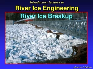
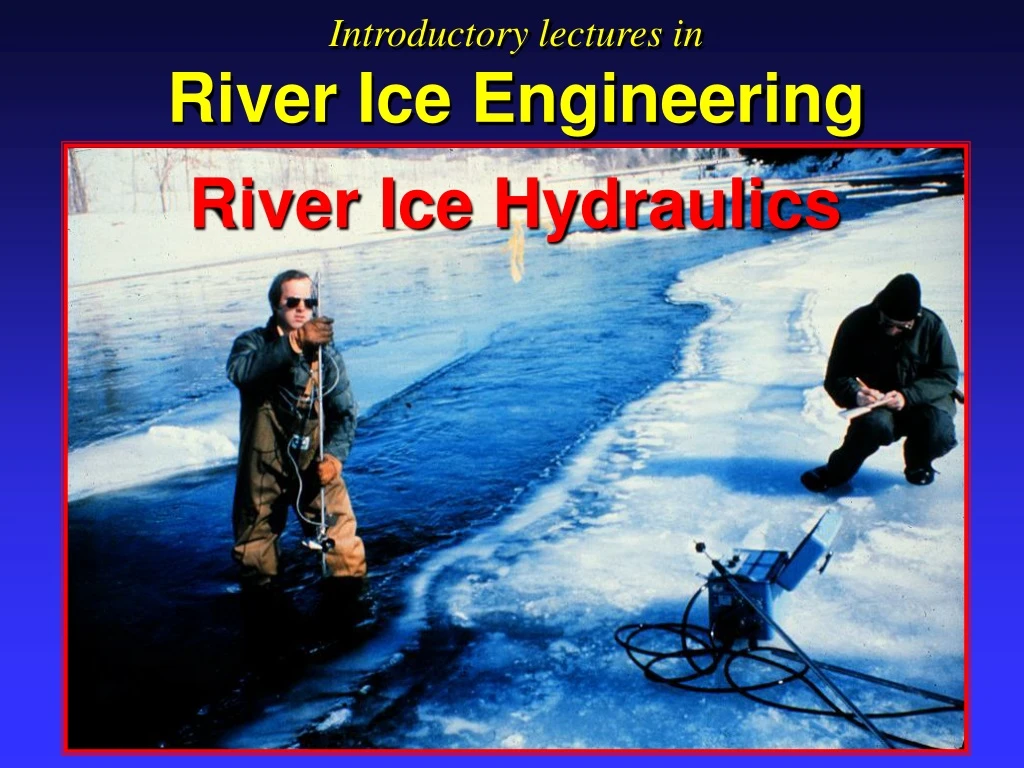
1. Introductory lectures in River Ice Engineering River Ice Hydraulics

2. Effects of Ice on the Flow • River ice floats with about 90% of its thickness submerged • this reduces the active flow area • River ice resists the flow of water • wetted perimeter is approximately doubled For an ice cover with underside roughness equal to the bed roughness, the water level will be about 30% higher than for the same discharge under open water conditions.

3. Mackenzie River at Fort Providence, 1994 (Hicks et al, 1995, data source, Water Survey of Canada)

4. Effects of the Flow on the Ice • under turning pans • consolidation or shoving (ice jams) THICKER ICE COVERS UNSTEADY FLOW

5. Complications to consider… photo source: R. Gerard

6. Open water rating curves are not applicable under ice affected conditions… Mackenzie River (Hicks et al., 1993) ice affected conditions ~1.5m open water conditions

7. Liard River above Fort Simpson (source WSC) (Hicks et al., 2000)

8. (Hicks et al., 2000)

9. Roughness of the underside of the ice cover is difficult to measure directly, or to deduce indirectly from velocity profiles… This ice floe has been turned over, to view the ripples on the underside. These ripples formed due to warm water flowing under the ice cover. photo by F. Hicks

10. February 23, 1978 February 16, 1978 Frazil slush may be obstructing the waterway… Ottauquechee River from Resistance coefficients from velocity profiles in ice-covered shallow streams” by Calkins, Deck and Martinson, CJCE, Vol. 9, Number 2, 1982

11. Peace River at Peace River, March 9, 1999 Preliminary WSC data (Hicks et al., 2000)

12. There may only be a partial ice cover… photo by S. Beltaos

13. Hydraulics of Ice Covered Channels Longitudinal Velocity Profile ICE BED (Ashton, 1986)

14. Composite Roughness Approach The channel cross section is divided into two sub-sections, one affected only by the ice, and one affected only by the bed. ice affected area bed affected area (Ashton, 1986)

15. General practice is to assume the line of zero shear, which divides the two subsections is coincident with the isoline of maximum velocity. ice affected area bed affected area (Ashton, 1986) This is actually true only if ni= nb

16. Common practice is to use Sabaneev’s equation to determine a composite roughness. valid for nb£ 0.04 and depth > 2m with an accuracy of 1% or better (Ashton, 1986) nb is for the rougher of two boundaries

17. Ice Jam Roughness (adapted from Ashton, 1986) ice roughness on the underside of ice jams can be as high as ni = 0.05 to 0.09 --- the use of Sabaneev’s equation here will be inaccurate…

18. Ice Jam Hydraulics there is currently no “model” for jam toe configuration (adapted from Beltaos, 1995) If the jam is sufficiently long, and the channel geometry is not highly variable, an ‘equilibrium section’ may form.

19. The equilibrium section is significant, since it is currently believed that it produces the maximum depth within the ice jam profile. (adapted from Ashton, 1986)

20. A non-dimensional depth versus discharge relationship for equilibrium conditions was developed by Beltaos (1983): handxrepresent the non-dimensional depth and discharge, respectively, and are defined as : B = accumulation width S= stream slope q= discharge per unit width h = flow depth from the water surface to the bed ( depth of flow below the ice cover plus the submerged ice thickness).

21. mis a jam strength parameter, typically ranging from 0.9 to 1.3 K.D. White, CRREL Report 99-11

22. Cohesion is assumed to be negligible (a conservative assumption). fois the composite friction factor for the flow under an ice jam: fi and fb denote the friction factors for the ice and bed influenced portions of flow, respectively. Arguing the insensitivity of his relationship to variations in friction factor (due to the small exponent), Beltaos introduced the following non-dimensional graph forh versusx

23. All points are based on actual field data. x known only as a range Scatter in the diagram is due to variation in friction factor. (adapted from Ashton, 1986)

24. …due to variation in friction factor (Beltaos, 1995)

25. Example calculation of water depth associated with equilibrium jam conditions: • GIVEN: • B = accumulation width = 50 m • S= stream slope = 0.0002 • q= discharge per unit width = 1 m3/s/m • FIND: • h = flow depth from the water surface to the bed. First, determine x,the non-dimensional discharge, using:

26. 250 (Beltaos, 1995)

27. From the graph, h, the non-dimensional depth equals 250: Now, we can determine the flow depth, h, using: The maximum flow depth, associated with the equilibrium section of the ice jam, would be 2.5 m. Note also though, the scatter in the observed data indicated that h could range from about 230 to 280, so h could be anywhere from 2.3 to 2.8 m. (The variation is due to the fact that roughness is not accounted for in this calculation.)

28. Ice Jam ModellingThis is the preferred approach for most applications… (adapted from Ashton, 1986)

29. Ice Jam Models • RIVJAM • S. Beltaos, National Water Research Institute • ICEJAM • Flato and Gerard, University of Alberta • HEC-RAS (U.S. Army Corps of Engineers) • Daly, Cold Regions Research and Engineering Laboratory (based on ICEJAM model) • http://www.hec.usace.army.mil/software/software_distrib/hec-ras/hecrasprogram.html To learn about ice jam modelling with RIVJAM and ICEJAM see the paper by Healy and Hicks in the ASCE Journal of Cold Regions Engineering (1999, Vol. 13, No. 4, pp. 180-198).