Introduction to Differential Expression Analysis
Introduction to Differential Expression Analysis. Microarray Experiment Steps. Biological question. Experimental design. Microarray experiment. Database. Data Analysis. Biological verification and interpretation. Most Common Types of Data Analysis.

Introduction to Differential Expression Analysis
E N D
Presentation Transcript
Microarray Experiment Steps Biological question Experimental design Microarray experiment Database Data Analysis Biological verification and interpretation
Most Common Types of Data Analysis • Class Discovery (Clustering, Unsupervised learning) • Class Prediction (Classification, Supervised Learning) • Class Comparison (Differential Expression)
Outline • Differential expression experiments • First look at microarray data • Data transformations and basic plots • General statistical issues
Differential Expression • Many microarray experiments are carried out to find genes which are differentially expressed between two (or more) samples of cells. Examples abound! • Initially, comparative microarray experiments were done with few, if any replicates, and statistical criteria were not used for identifying differentially expressed genes. Instead, simple criteria were used such as fold-change, with 2-fold being a popular cut-off. • The simplest experiment involves comparing two samples on one array with two-color technology or two arrays if using one-color technology
Why logs? • For better of worst, fold changes are the preferred quantification of differential expression. Fold changes are basically ratios • Biologist sometimes use the following weird notation: -2 means 1/2, -3 means 1/3, etc… Note there are no values between -1 and 1! • Ratios are not symmetric around 1. This makes it problematic to perform statistical operations with ratios. We prefer logs
Why logs • The intensity distribution has a fat right tail • Log of ratios are symmetric around 0: • Average of 1/10 and 10 is about 5 • Average of log(1/10) and 10 is 0 • Averaging ratios is almost always a bad idea! Facts you must remember: log(1) = 0 log(XY) = log(X) + log(Y) log(Y/X) = log(Y) - log(X) log(√X) = 1/2 log(X)
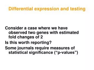
Example • Consider a case were we have observed two genes with fold changes of 2 • Is this worth reporting? Some journals require statistical significance. What does this mean? * *
Review of Statistical Inference • Let Y-X be our measurement representing diferential expression • What is the typical null hypothesis? • For simplicity let us assume Y-X follows a normal distribution • Y-X may have a different distribution under the null hypothesis for different genes • More specifically the standard deviation of Y-X may be different. • We could consider (Y-X) / instead • But we do not know ! • What is ? Why is it not 0? • How about taking samples and using the t-statistic?
Sample Summaries Observations: Averages: SD2 or variances:
The t-statistic t - statistic:
Properties of t-statistic • If the number of replicates is very large the t-statistic is normally distributed with mean 0 and and SD of 1 • If the observed data is normally distributed then the t-statistic follows a t distribution regardless of sample size • We can then compute probability that t-statistic is as extreme or more when null hypothesis is true • Where does probability come from? • We will see that using the t-statistic is not a good strategy for microarray data when N is small
Inference of Ranking • Are we really interested in inference? • Sometimes all we are after is a list of candidate genes • If we are just ranking should we still consider variance?
A 45 rotation highlights a problem This is referred to as MAplot
Experiments with replicates • If we are interested in genes with over-all large fold changes why not look at average (log) fold changes? • Experience has shown that one usually wants to stratify by over-all expression • We can make averaged MA plots: • M = difference in average log intensities and • A = average of log intensities
How do we summarize? • Seems that we should consider variance even if not interested in inference • The t-test is the most used summary of effect size and within population variation
The volcano plot shows, for a particular test, negative log p-value against the effect size (M) Another useful plot
Estimating the variance • If different genes (or probes) have different variation then it is not a good idea to use average log ratios even if we do not care about significance • Under a random model we need to estimate the SE • The t-test divides by SE • But with few replicates, estimates of SE are not stable • This explains why t-test is not powerful • There are many proposals for estimating variation • Many borrow strength across genes • Empirical Bayesian Approaches are popular • SAM, an ad-hoc procedure, is even more popular • Many are what some call “moderated” t-tests • More in later lecture
Say we are interested in statistical inference, we need to define statistical significance. If we are ranking we may need to define a cut-off that defines interesting enough The naïve answer to determinig a cut-off is the p-values. Are they appropriate? Test for each gene null hypothesis: no differential expression. Notice that if you have look at 10,000 genes for which the null is true you expect to see 500 attain p-values of 0.05 This is called the multiple comparison problem. Statisticians fight about it. But not about the above. Main message: p-values can’t be interpreted in the usual way A popular solution is to report FDR instead. One final problem
What do we do? • Adjusted p-values • List of genes along with FDR • Bayesian inference • Forget about inference: use EDA • We may talk about this in detail in another lecture
Multiple Hypothesis Testing • What happens if we call all genes significant with p-values ≤ 0.05, for example? Null = Equivalent Expression; Alternative = Differential Expression
Error Rates • Per comparison error rate (PCER): the expected value of the number of Type I errors over the number of hypotheses PCER = E(V)/m • Per family error rate (PFER): the expected number of Type I errors PFER = E(V) • Family-wise error rate: the probability of at least one Type I error FEWR = Pr(V ≥ 1) • False discovery rate (FDR) rate that false discoveries occur FDR = E(V/R; R>0) = E(V/R | R>0)Pr(R>0) • Positive false discovery rate (pFDR): rate that discoveries are false pFDR = E(V/R | R>0) • More later.