Predicting Exchange Rate Volatility Using Genetic Programming: An Innovative Approach
430 likes | 550 Views
This paper investigates the application of a genetic programming model as a non-parametric method for forecasting exchange rate volatility, focusing on the Dollar against the German Mark and Japanese Yen. The study highlights the strengths of genetic programming in detecting complex patterns in financial data that traditional models overlook. Results indicate the efficacy of this approach while also addressing challenges such as overfitting. The paper outlines data implementation, experimental designs, and performance evaluation against benchmark models like GARCH, offering insights into the predictive capabilities for financial markets.

Predicting Exchange Rate Volatility Using Genetic Programming: An Innovative Approach
E N D
Presentation Transcript
USING A GENETIC PROGRAM TO PREDICT EXCHANGE RATE VOLATILITY Christopher J. Neely Paul A. Weller
Outline • Introduction • The Genetic Program • Data and Implementation • Experimental Designs • Results • Conclusion • Discussion
Introduction • Exchange rate volatility displays considerable persistence. • Large movements in prices tend to be followed by more large moves, producing positive serial correlation in absolute or squared returns. • Engle (1982) ARCH model • Bollerslev (1986) GARCH model • This paper investigates the performance of a genetic program as a non-parametric procedure for forecasting volatility in the foreign exchange market.
Strength and Weakness • Strength • Genetic programs have the ability to detect patterns in the conditional mean of foreign exchange and equity returns that are not accounted for by standard statistical models (Neely, Weller, and Dittmar 1997; Neely and Weller 1999 and 2001; Neely 2000). • Weakness • Over fitting
The Genetic Program • Function Set • Data functions • data, average, max, min, and lag. • Four data series • Three more complex data functions • geo, mem, arch5 • An Example of a GP Tree • Volatility
Function Set • plus, minus, times, divide, norm, log, exponential, square root, and cumulative standard normal distribution function.
Four data series • Daily Returns • Integrated Volatility • the sum of squared intraday returns • The sum of the absolute value of intraday returns • Number of days until the next business day
The function geo returns the following weighted average of 10 lags of past data. • This function can be derived from the prediction of an IGARCH specification with parameter , where we constrain to satisfy 0.01 0.99 and lags are truncated at 10.
The function mem returns a weighted sum similar to that which would be obtained from a long memory specification. • j>0 hj=1 • d is determined by the genetic program and constrained to satisfy -1< d <1.
The function arch5 permits a flexible weighting of the five previous observations. • hjare provided by the genetic program and constrained to lie within {-5,5} and to sum to one.
Volatility • Since true volatility is not directly observed, it is necessary to use an appropriate proxy in order to assess the performance of the genetic program. • Use the ex post squared daily return. • Andersen and Bollerslev (1998) • A better approach is to sum intraday returns to more accurately measure true daily volatility (i.e.,integrated volatility).
Si,t is the i-th observation on date t • 2i,tis the measure of integrated volatility on date t. • More precisely, daily volatility is calculated from 1700 GMT to 1700 GMT. • Using five intraday observations represents a compromise between the increase in accuracy generated by more frequent observations and the problems of data handling and availability that arise as one moves to progressively higher frequencies of intraday observation.
Data and Implementation • Dollar / German mark (DEM) • Dollar / Japanese yen (JPY) • June 1975 to September 1999. • Training period June 1975 – December 1979 • Selection period January 1980 – December 30, 1986 • Out-of-sample period December 31, 1986 – September 21, 1999 • The sources of the data • Step
Step • Create an initial generation of 500 randomly generated forecast functions. • Measure the MSE of each function over the training period and rank according to performance. • Select the function with the lowest MSE and calculate its MSE over the selection period. Save it as the initial best forecast function. • Select two functions at random, using weights attaching higher probability to more highly-ranked functions. Apply the recombination operator to create a new function, which then replaces an old function, chosen using weights attaching higher probability to less highly-ranked functions. Repeat this procedure 500 times to create a new generation of functions.
Measure the MSE of each function in the new generation over the training period. Take the best function in the training period and evaluate the MSE over the selection period. If it outperforms the previous best forecast, save it as the new best forecast function. • Stop if no new best function appears for 25 generations, or after 50 generations. Otherwise, return to stage 4.
Experimental Designs • Benchmark • Fitness Function • Measure of Forecast Errors • Forecasts Aggregation • Other Designs
Benchmark • GARCH (1,1)
Fitness Function • MSE • MSE + Penalty
Overfitting • Penalty Function for Node Complexity • This consisted of subtracting an amount (0.002 * number of nodes) from the negative MSE. This modification is intended to bias the search toward functions with fewer nodes, which are simpler and therefore less prone to overfit the data.
Measure of Forecast Errors • mean square error • mean absolute error • R-square • mean forecast bias • kernel estimates of the error densities.
Forecasts Aggregation • The forecasts were aggregated in one of two ways. • Mean: The equally-weighted forecast is the arithmetic average of the forecasts from each of the ten trials. • Median: The median-weighted forecast takes the median forecast from the set of ten forecasts at each date.
Other Designs • forecast horizon: 1, 5, 10 • the number of data functions: 5, 8 • penalty for complexity: absent, present
Results • An example of a one-day ahead forecasting functions for the DEM • In-sample comparison of GP and GARCH • Out-of- sample comparison of GP and GARCH • Out-of- sample results using the data functions geo, mem, arch5 • Kernel estimates of the densities of out-of sample forecast errors • Tests for mean forecast bias -- Newey-West correction for serial correlation • Summary
In-sample comparison of GP and GARCH • The equally-weighted forecast is the arithmetic average of the forecasts from each of the ten trials. • The median-weighted forecast takes the median forecast from the set of ten forecasts at each date.
In-Sample • That is, its best relative performance is at the twenty-day horizon. • The median weighted forecast is generally somewhat inferior to the equally weighted forecast.
< < < < Out-of- sample comparison of GP and GARCH
Out-of-Sample • With MSE as the performance criterion, neither the genetic program nor the GARCH model is clearly superior. • The GARCH model achieves higher R^2 in each case. • But the MAE criterion clearly prefers the genetic programming forecasts.
Out-of- sample results using the data functions geo, mem, arch5
Effect of Advanced Functions • We have established that neither imposing a penalty for complexity nor expanding the set of data functions leads to any appreciable improvement in the performance of the genetic program.
Effect of the Penalty Function • This had very little effect and if anything led to a slight deterioration in out-of-sample performance.
Kernel estimates of the densities of out-of sample forecast errors The appearance of greater bias in the GARCH forecasts is illusory.
The most striking feature to emerge from these figures is the apparent bias in the GARCH forecasts when compared to their genetic program counterparts.
Tests for mean forecast bias • Though both forecasts are biased in the mean, the magnitude of the bias is considerably greater for the genetic program.
Summary • While the genetic programming rules did not usually match the GARCH(1,1) model's MSE or R^2 at 1-and 5-day horizons, its performance on those measures was generally close. • But the genetic program did consistently outperform the GARCH model on mean absolute error (MAE) and modal error bias at all horizons and on most measures at 20-day horizons.
Conclusion • GP did reasonably well in forecasting out-of-sample volatility. • While the GP rules did not usually match the GARCH(1,1) model’s MSE or R2 at 1- and 5-day horizons, its performance on those measures was generally close. • GP did consistently outperform the GARCH model on mean absolute error (MAE) and modal error bias at all horizons and on most measures at 20-day horizons.
Discussion • Choice of Function Sets • Simple Functions (Primitive Functions) • Complex Functions • Use of Data Functions • True Volatility • The Selection Period
Use of Data Functions • The data functions can operate on any of the four data series we permit as inputs to the genetic program. • data, average, max, min, and lag.
True Volatility • The functions generated by the genetic program produce forecasts of volatility. • Since true volatility is not directly observed, it is necessary to use an appropriate proxy in order to assess the performance of the genetic program.
The Selection Period • What is the difference between Neely’s GP and the regular GP? • Neely introduced a new termination criterion, which is based on the recent progress. This idea itself is not new. • What makes Neely’s idea unique is that the progress is measured by a ``testing sample’’, which he called it the selection period.
The Selection Period • Neely’s GP can be considered as another approach to avoid over-fitting. • Because one characteristic of over fitting is the feature that the in-sample performance is improving, while the post-sample performance is stagnated or get worse. • Use Szpiro (2001)’s three-stage development of GP in data mining as a reference. • This is similar to the early stopping criterion frequently used in the artificial neural nets.