Transformations
Learn about transforming non-normal data, relevant methods, and how to apply transformations to achieve linear models. Discover common transformations like logarithms and roots, as well as advanced methods such as exponential and power functions.

Transformations
E N D
Presentation Transcript
Transformations Getting normal or using the linear model
Two Reasons to Transform • Variables do not fit a normal distribution and parametric tests are desired • A relationship between two variables is non-linear but transformation would allow the use of linear regression
Non-Normal Data • Reasons real data can fail to follow a normal distribution: • Errors in measurement are multiplicative rather than additive, e.g. ± 2% rather than ± 2mm • Constraints on the dimensions of an artifact feature are not symmetrical, e.g. point length must exceed haft length but can be as long as the material allows
Non-Normal Data 2 • Measurements are products rather than sums of other measurements, e.g. area, volume • Counts follow binomial, poisson, or negative binomial distributions which are often asymmetrical unless sample sizes are large
Solutions • Use non-parametric methods that do not depend on the normality of the data (increasingly easy to do) • Use data transformations that shift the distribution to one that is normal
Transformation • The goal is to change the spacing of the data to compress a long tail and draw out a flat tail • The transformation must preserve the order of the original data – we only change the spacing between data points
Transformation • Right skewed data with many zeros cannot be transformed effectively since nothing can stretch out observations that have the same value – e.g. artifact counts by site, grid square are often poisson distributed with many zeros
An Example • Using the DartPoints data set, we saw that Length was asymmetrical • Plot the kernel density of Length with and without a log scale to see the difference • To transform Length we would use • logLength <- log(DartPoints$Length)
plot(density(DartPoints$Length), main="Dart Point Length", xlab="Normal scale") plot(density(DartPoints$Length), main="Dart Point Length", xlab="Log scale", log="x")
Common Transformations • Tail to the right • Natural or common (base 10) logarithm – no zero values • Square root, cube root, etc – zeros ok • Inverse, -1/x, -1/x2, etc – no zero values • Tail to the left • Exponential ex,10x (low values) • Square, cube, etc
Other Transformations • arctangent (inverse tangent) to handle values between 0 and 1 used for population studies of non-metric traits
Transforming to Linear • By transforming variables before using linear regression we can fit nonlinear equations • In some cases we can express the fitted equation in terms of the original untransformed variables
Polynomial • Y = a + b1x + b2x2 + b3x3 + b4x4 . . . • Create polynomial values or use the function poly() within lm() • Begin with linear and then work up to quadratic, cubic, and so on until the new terms are not significant • Eg. lm(y~x+I(x^2)+I(x^3))
Power Function • Log-log transformation • Use log() to transform dependent and independent variables • Compute linear regression • log(y) = a + b * log(x) • y = Axb (where A= exp(a)) • If b = 1, same as the linear model • x, y > 0
Exponential function • Semi-log transformation • Use log() to transform dependent variable, y > 0 • Compute linear regression • log(y) = a + b * x • y = Aebx (where A= exp(a)) • Fits data with asymptotes
Inverse Function • Reciprocal transformation – 1/x where x ≠ 0 • Used for distance models – marriage, trade, social interaction declines with distance • Fits data with asymptotes
Other Functions • Logarithmic – no zeros in x • y = a + b * log(x) • Square Root – no negative values in x • y = a + b * sqrt(x)
Examples • Human cranial capacity over the last 1.8 million years • Number of Identified Specimens (NISP) and Minimum Number of Individuals (MNI) at Chucalissa (Middle Misssissippian site)
# BrainsCC.RData # Explore logs with scatterplot RegModel.1 <- lm(BrainCC~AgeKa, data=BrainsCC) # Rcmdr summary(RegModel.1) # Rcmdr BrainsCC$logAge <- with(BrainsCC, log(AgeKa)) # Rcmdr BrainsCC$logBrain <- with(BrainsCC, log(BrainCC)) # Rcmdr RegModel.2 <- lm(logBrain~logAge, data=BrainsCC) # Rcmdr summary(RegModel.2) # Rcmdr RegModel.3 <- lm(BrainCC~logAge, data=BrainsCC) # Rcmdr summary(RegModel.3) # Rcmdr plot(BrainCC~AgeKa, data=BrainsCC, pch="+") abline(RegModel.1, lty=1, lwd=2, col="black") x <- seq(0, 1800, 10) logx <- log(x) lines(x, exp(predict(RegModel.2, data.frame(logAge=logx))), lty=1, lwd=2, col="red") lines(x, predict(RegModel.3, data.frame(logAge=logx)), lty=1, lwd=2, col="blue") legend("topright", c("Linear", "Power", "Logarithmic"), lty=1, lwd=2, col=c("black", "red", "blue"))
LinearModel.4 <- lm(BrainCC ~ AgeKa + I(AgeKa^2), data=BrainsCC) summary(LinearModel.4) LinearModel.5 <- lm(BrainCC ~ AgeKa + I(AgeKa^2) + I(AgeKa^3), data=BrainsCC) summary(LinearModel.5) LinearModel.6 <- lm(BrainCC ~ AgeKa + I(AgeKa^2) + I(AgeKa^3) + I(AgeKa^4), data=BrainsCC) summary(LinearModel.6) plot(BrainCC~AgeKa, data=BrainsCC, pch="+") abline(RegModel.1, lty=1, lwd=2, col="black") x <- seq(0, 1800, 10) lines(x, predict(LinearModel.4, data.frame(AgeKa=x)), lty=1, lwd=2, col="red") lines(x, predict(LinearModel.5, data.frame(AgeKa=x)), lty=1, lwd=2, col="blue") lines(x, predict(LinearModel.6, data.frame(AgeKa=x)), lty=1, lwd=2, col="green") legend("topright", c("Linear", "Quadratic", "Cubic", "Quartic"), lty=1, lwd=2, col=c("black", "red", "blue", "green"))
load("C:/Users/DCarlson/Documents/anth642/R/Data/Chucalissa.rda") #Rcmdr plot(mni~nisp, data=Chucalissa) RegModel.1 <- lm(mni~nisp, data=Chucalissa) #Rcmdr summary(RegModel.1) #Rcmdr abline(RegModel.1) plot(mni~nisp, data=Chucalissa, log="xy") # Plot log-log transform plot(mni~nisp, data=Chucalissa, log="y") # Plot semi-log transform Chucalissa$logMNI <- log(Chucalissa$mni) # Create logged variables Chucalissa$logNISP <- log(Chucalissa$nisp) plot(logMNI~logNISP, data=Chucalissa) RegModel.2 <- lm(logMNI~logNISP, data=Chucalissa) #Rcmdr summary(RegModel.2) #Rcmdr abline(RegModel.2) plot(mni~nisp, data=Chucalissa) # plot log-log equation on original data a2 <- exp(RegModel.2$coefficients[[1]]) # Convert a to exp(a) b2 <- RegModel.2$coefficients[[2]] a1 <- RegModel.1$coefficients[[1]] b1 <- RegModel.1$coefficients[[2]] curve(a2*x^b2, 0, 3250, add=TRUE) abline(RegModel.1, lty=3) text(locator(), as.expression(substitute(MNI == a*NISP^b, list(a=round(a2, 4), b=round(b2, 4)))), pos=2) text(locator(), as.expression(substitute(MNI == a+b*NISP, list(a=round(a1, 4), b=round(b1, 4)))), pos=4)