Nonlinear Dimensionality Reduction Approach (ISOMAP, LLE)

1. Nonlinear Dimensionality Reduction Approach(ISOMAP, LLE) Young Ki Baik Computer Vision Lab. SNU

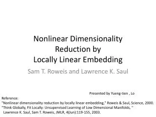
2. References • ISOMAP • A global geometric framework for nonlinear dimensionality reduction • J.B.Tenenbaum, V.De Silva, J.C.Langford (science 2000) • LLE • Nonlinear Dimensionality Reduction by Locally Linear Embedding • Sam T. Roweis and Lawrence K. Saul (science 2000) • ISOMAP and LLE • LLE and Isomap Analysis of Spectra and Colour Images • Dejan Kulpinski (Thesis 1999) • Out-of-Sample Extensions for LLE, Isomap, MDS, Eignemaps, and Spectral Clustering • Yoshua Bengio et. Al. (TR2003)

3. Contents • Introduction • PCA and MDS • ISOMAP and LLE • Conclusion

4. Dimensionality Reduction • Problem • Complex stimuli can be represented by points in a high-dimensional vector space. • They typically have a much more compact description. • The goal • The meaningful low-dimensional structures hidden in their high-dimensional observations in order to compress the signals in size and discover compact representations of their variable.

5. Dimensionality Reduction • Simple example • 3-D data

6. Dimensionality Reduction • Linear method • PCA (Principle Component Analysis) • Preserves the variance • MDS (Multi Dimensional Scaling) • Preserves inter-point distance • Non-linear method • ISOMAP • LLE • …

7. Linear Dimensionality Reduction • PCA • Find a low-dimensional embedding of the data points that best preserves their variance as measured in the high-dimensional input space. • Eigenvectors are the principal directions, and eigen- values represent the variance of the data along each principal direction. is the marginal variance along the principle direction

8. Linear Dimensionality Reduction • PCA • Projecting onto e1 captures the majority of the variance and hence it minimizes the error. • Choosing subspace dimension M: • Large M means lower expected error in the subspace data approximation Reduction

9. Linear Dimensionality Reduction • MDS • Find an embedding that preserves the inter-point distances, equivalent to PCA when the distances are Euclidean. PCA MDS

10. Linear Dimensionality Reduction • MDS • distances • Relation

11. Linear Dimensionality Reduction • MDS • Providing dimension reduction. • Relating tools Method 1 PCA MDS Method 2 Dimension Reduction Method …

12. Nonlinear Dimensionality Reduction • Many data sets contain essential nonlinear structures that invisible to PCA and MDS. • Resort to some nonlinear dimensionality reduction approaches.

13. ISOMAP • Example of non-linear structure(swiss roll) • Only the geodesic distances reflect the true low-dimensional geometry of the manifold. • ISOMAP (Isometric feature Mapping) • Preserves the intrinsic geometry of the data. • Uses the geodesic manifold distances between all pairs.

14. ISOMAP (algorithm description) • Step 1 • Determining neighboring points within a fixed radius based on the input space distance • These neighborhood relation are represented as a weighted graph G over the data points. • Step 2 • Estimating the geodesic distances between all pairs of points on the manifold by computing their shortest path distances in the graph G. • Step 3 • Constructing an embedding of the data in d-dimensional Euclidean space Y that best preserves the manifold’s geometry.

15. ISOMAP (algorithm description) • Step 1 • Determining neighboring points within a fixed radius based on the input space distance # ε-radius# K-nearest neighbors • These neighborhood relationsare represented as a weighted graph G over the data points. K=4 ε i j k

16. ISOMAP (algorithm description) • Step 2 • Estimating the geodesic distances between all pairs of points on the manifold by computing their shortest path distances in the graph G. • Can be done using Floyd’s algorithm or Dijkstra’s algorithm j i k

17. Solution: take top d eigenvectors of the matrix ISOMAP (algorithm description) • Step 3 • Constructing an embedding of the data in d-dimensional Euclidean space Y that best preserves the manifold’s geometry. • Minimize the cost function

18. Manifold Recovery Guarantee of ISOMAP • Isomap is guaranteed asymptotically to recover the true dimensionality and geometric structure of nonlinear manifolds. • As the sample data points increases, the graph distances provide increasingly better approximations to the intrinsic geodesic distances.

19. Experimental Results (ISOMAP) # Face # Hand writing : face pose and illumination : bottom loop and top arch MDS : open triangles Isomap : filled circles

20. LLE • LLE (Locally Linear Embedding) • Neighborhood preserving embeddings. • Mapping to global coordinate system of low dimensionality. • Recovering global nonlinear structure from locally linear fits. • Each data point and it’s neighbors is expected to lie on or close to a locally linear patch. • Each data point is constructed by it’s neighbors: • Where Wij summarize the contribution of j-th data point to the i-th data reconstruction and is what we will estimated by optimizing the error. • Reconstructed from only its neighbors.

21. LLE (algorithm description) • We want to minimize the error function • With the constraints : • Solution (using lagrange multipliers):

22. Quadratic form: where: LLE (algorithm description) • Choose d-dimensional coordinates, Y, to minimize: • Under : • Solution : compute bottom d+1 eigenvectors of M. (discard the last one)

23. LLE (algorithm summary) • Step 1 • Compute the neighbors of each data point, Xi • Step 2 • Compute the weight Wij that best reconstruct each data point Xifrom its neighbors, minimizing the cost in eq(1) by constrainted linear fits. • Step 3 • Compute the vectors Yibest reconstructed by the weights Wij, minimizing the quadratic form in eq(2) by its bottom nonzero eigenvectors. 1 2

24. Experimental Results (LLE) • Lips # PCA # LLE

25. Conclusion • ISOMAP • Use the geodesic manifold distances between all pairs. • LLE • Recovers global nonlinear structure from locally linear fits. • ISOMAP vs LLE • Preserving the neighborhoods and their geometric relation. • LLE requires massive input data sets and it must have same weight dimension. • Merit of Isomap is fast processing time with dijkstra’s algorithm. • Isomap is more practical than LLE.