Download
1 / 26
260 likes | 399 Views
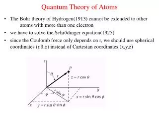
The Quantum Theory of Atoms and Molecules. Breakdown of classical physics: Wave-particle duality Dr Grant Ritchie. Electromagnetic waves. Remember : The speed of a wave, v , is related to its wavelength, , and frequency, f , by the relationship v = f .

E N D
The Quantum Theory ofAtoms and Molecules Breakdown of classical physics: Wave-particle duality Dr Grant Ritchie
Electromagnetic waves Remember: The speed of a wave, v, is related to its wavelength, , and frequency, f, by the relationship v=f. Speed of the em wave in vacuum is a fundamental constant, with the value c2.998108ms1. Faraday’s law of induction: A time-varying magnetic field produces an electric field. Maxwell showed that the magnetic counterpart to Faraday’s law exists, i.e. a changing electric field produces a magnetic field, and concluded that em waves have both electric, E, and magnetic, B, components.
Principle of superposition Particles bounce off or stick together when they collide, where as waves pass through unhindered. While there can be interference effects in the region of overlap (see later), the characteristics of two waves after an interaction is the same as before they came together. The resultant distortion due to the combination of several waves 1, 2, 3,…, is just given by their sum: For the case of two waves, =1+2 : where the crests and troughs of 1 match up with those of 2 respectively, there is an enhancement due to constructive interference; when there is a mismatch, so that the high points of 1 overlap with the low ones of 2, there is a net reduction in the magnitude of the wave due to destructive interference. Note: The energy carried by a wave is proportional to the square of the amplitude, 2=* and this usually determines what is measured experimentally; for 2 component case, that is 1 + 22. See later on the double slit experiment with both light and particles.
Interference Superposition of two linearly polarised waves, E1 and E2, of the same frequency leads to a wave with the following electric field distribution, Eres : The amplitude factor dependent upon the phase difference=(12) between components: Largest resultant amplitude when =n2 (n is an integer) total constructive interference; By contrast, resultant wave has zero amplitude if =(2n +1) total destructive interference.
Young's double slit experiment Light from single source passes through pinhole and illuminates two narrow slits separated by a distance d. - WHY? Interference pattern is observed on screen (distance D after slits) due to the superposition of waves originating from bothslits. Point P has maximum intensity if the two beams are totally in phase at that pointso the condition for total constructive interference is: * We have restated the condition for constructive interference as the case where the optical path difference (OPD)between the component waves is an integral number of wavelengths. OPD and are related as follows:
Young’s slits continued By assuming that Dy,d then Position on screen: so that separation between adjacent maxima: Maxima occur at: Young's double slit experiment is an example of interference by division of wavefront. Definitely a wave phenomenon!
Diffraction Diffraction is the bending of light at the edges of objects. Light passing through aperture and impinging upon a screen beyond has intensity distribution that can be calculated by invoking Huygen’s principle. Wavefront at the diffracting aperture can be treated as a source of secondary spherical wavelets.
The single slit Consider point P and rays that originate from the top of the slit and the centre of the slit respectively. If the path difference (asin)/2 between these two rays is /2, then the two rays will arrive at point Pcompletely out of phase and will produce no intensity at that point. For any ray originating from a general point in the upper half of the slit there is always a corresponding point distance a/2 away in the lower half of the slit that can produce a ray that will destructively interfere with it. Thus the point P, will have zero intensity and is the first minimum of the diffraction pattern. The condition for the first minimum is
The single slit continued In general a minimum occurs when path difference between the rays at A and B (separated by the distance a/2) is an odd number of half-wavelengths; i.e. (m1/2)/2 where m=1, 2, 3,,. The general expression for the minima in the diffraction pattern is thus For light of a constant wavelength the central maximum becomes wider as the slit is made narrower. The intensity distribution of diffracted light, Ires, is This characteristic distribution is known as a sincfunction. The maximum value of this function occurs at =0 and has zero values when =,2,..,n. Another example of a wave phenomenon!
Photons EM radiation is not continuous, in the sense that the total energy cannot take any arbitrary value it is quantised. The smallest unit of EM radiation is the photon and has the energy E = h where h is Planck’s constant (= 6.626 1034 J s). • Evidence: • Thermal/Blackbody radiation • Photoelectric effect • 3.Spectroscopy – with quantised energy levels in atoms and molecules, spectroscopic transitions can only occur at discrete frequencies, i.e. with well defined energies of the photons. • As well as possessing a well defined energy, photons also exhibit • momentum, p = h/c = h/ = kh/2. – the Compton effect, radiation pressure. • angular momentum with a value of + h/2 or h/2 around the direction of motion corresponding to right and left circularly polarised light. (See atomic spectroscopy lectures - for example, transitions between two s orbitals are forbidden).
Thermal radiation I Radiation that is given out by a body as a result of its temperature. e.g humans emit infrared Total rate of radiation T 4 (Stefan’s Law). Spectrum shifts to shorter wavelengths as T increases (maxT = const – Wien’s law).
Thermal radiation II Black body spectrum calculated by Rayleigh and Jeans (1900). Experiment and theory disagree – Ultraviolet catastrophe. Planck:Light comes in photons E = nh where n = 1, 2, 3,…. Short wavelength photons have too much energy to be supplied by thermal motions with energy kT. (h >> kT) Rayleigh assumed that every wavelength carried kT in energy (equipartition). Planck explained the form of the thermal spectrum successfully but had to (i) throw out the wave picture of light, and (ii) introduce a new fundamental constant, h.
The Photoelectric effect Light shining onto matter causes the emission of photoelectrons. Note: 1. Photoelectrons are emitted instantly, whatever the intensity of the light. 2. There is a critical frequency below which no photoelectrons are emitted. 3. Maximum kinetic energy of photoelectrons increases linearly with frequency. Planck’s photon picture: E = h. The photon supplies the energy available, = hc (ionisation energy / work function) For < c, not enough energy to ionise. For > c, hc used in ionisation, the rest is carried off by the electron as kinetic energy: KEmax = h . Basis of photoelectron spectroscopy.
The Compton effect Compton measured intensity of scattered X-rays from a solid target as a function of for different angles. Observation: Peak in scattered radiation shifts tolonger wavelengths than source. Amount depends on (but not on target material) Classical picture: Oscillating EM field causes oscillations in positions of charged particles, which re-radiate in all directions at same frequency and wavelength as the incident radiation no wavelength shift! Momentum and energy conservation applied to collision between the photon and the electron gives correct results IF momentum of X-ray photons is p = h/!
The Compton Effect c is the Compton wavelength = 2.4 1012 m. NB. At all angles there is also an unshifted peak and this is due to a collision between the X-ray photon and the nucleus of the atom. For this case
Laser cooling Counterpropagating beams, every photon absorbed slows the atom down (re-emission is in a random direction). Laser beam molecular beam Stationary atoms give very sharp spectra (Doppler effect) Velocity distribution of laser cooled calcium atoms at (a) 3 mK and (b) 6 µK. Example: Na has an atomic absorption line at 589.6 nm. A Na atom, which is initially travelling at 400 m s-1 in the opposite direction to light of this wavelength, is brought to rest by the absorption of light. Calculate the number of photons absorbed. (Prelims 2003)
It get’s worse…..Matter waves Wave properties Wavelength, frequency Energy spread out over wavefront Interference Energy (amplitude)2 Light has both wave and particle characteristics: Particle properties Mass, position, velocity Energy localised at position of the particle No interference But particles can also have wave-like properties, with the wavelength related to the momentum p in the same way as for light: p = h / (de Broglie). Is this true?
electron beam interference pattern screen Electron diffraction Electrons have similar wavelength to atomic dimensions ( 1010 m) can use an array of atoms (crystal, metal foil) to produce an interference pattern with electrons and thus show that electrons have wave properties. The Davisson-Germer experiment (1927). Metal foil Example:Electrons, accelerated through a potential difference of 100V, can be diffracted by the layers of metal atoms in a metal crystal. Comment.
The double-slit experiment with….. •Performed with electrons C Jönsson 1961 Zeitschrift für Physik 161 454-474, (translated 1974 American Journal of Physics 42 4-11) •Performed with single electrons A Tonomura et al. 1989 American Journal of Physics 57 117-120 •Performed with neutrons A Zeilinger et al. 1988 Reviews of Modern Physics 60 1067-1073 •Performed with He atoms O Carnal and J Mlynek 1991 Physical Review Letters 66 2689-2692 •Performed with C60 molecules M Arndt et al. 1999 Nature 401 680-682 •Performed with C70 molecules L. Hackermüller et al 2004 Nature 427 711-714
1 2 2 slit single particle experiment Only slit 1 open P1 = y12 Only slit 2 open P2 = y22 Both slits open P12 = y12 + y22 + 2 y1y2 This observation is inexplicable in the particle picture.
Interpretation of the double slit experiment 1.The interference pattern consists of many independent events in which a particle is detected at a particular position in space on screen. A bright fringe indicates a high probability of particle being detected at that point while a dark fringe corresponds to low probability. 2.The fringe pattern required the presence of bothslits. Covering up one slit destroys the fringes. 3.Any attempt to determine which slit the particle passes through destroys the interference pattern. We cannot see the wave-particle nature at the same time. • 4.The flux of particles can be reduced so that only one particle arrives at a time interference fringes are still observed!. Thus, • Wave behaviour can be shown by a single atom; • Each particle goes through both slits at once; • c) A matter wave can interfere with itself. Observations also indicate that the process of measuring actually changes the system!
Single slit diffraction and the Heisenberg Uncertainty Principle Wave-like behaviour of electrons, atoms etc. leads to a fundamental loss of information about their position/momentum compare with a trajectory in classical mechanics. +x d p+x d q d q +y py = h/l d py d p-x l agrees with upper value of DxDpx≥ ħ/2 – x • px /py≈ q • q ≈ l/d = h / py d • Uncertainty through slit: x ≈ d / 2. px ~ h/d px x~ h/2 Uncertainty in momentum along x (introduced by -partially- locating position) Uncertainty in position along x We cannot have simultaneous knowledge of ‘conjugate’ variables such as position and momentum (in the same direction).
Dx How can a wave look like a particle? Add together two waves of the same amplitude but slightly different frequencies: If we let k1 = k k,k2 = k k and 1 = , 2 = + . The resultant is: Doesn’t look much like a particle!
Dx Dk k0 Wavepackets But can add more and more waves with slightly different wavevectors (different k values). Now wave is localised over a distance x wavepacket. Spatial extent of wavepacket x is inversely proportional to width of the distribution of wavevectors:
Heisenberg (again) Fourier analysis shows that kx 1. But de Broglie tells us that the uncertainty in the momentum is p = ħk, and so we arrive at the Heisenberg uncertainty principle: The wavepacket picture discussed is at a single time. If we view the wavepacket passing a fixed position, we will see a very similar disturbance as a function of time. Wavepacket in the time domain is made up of waves of different angular frequencies and its width in time tis related to the spread in frequencies by the relationship t 1. Multiplying by ħ we arrive at an energy-time uncertainty relation: Upshot: Transitions between energy levels of atoms/molecules are not perfectly sharp in frequency lifetime broadening. See later spectroscopy and photochemistry lectures.