Download
1 / 181
1.81k likes | 2.13k Views
Solving Classification Problems for Symptom Validity Tests with Mixed Groups Validation. Richard Frederick, Ph.D., ABPP (Forensic) US Medical Center for Federal Prisoners Springfield, Missouri. I am not a neuropsychologist. My view of brain. Your view of brain. My board certifications:.

E N D
Solving Classification Problems for Symptom Validity Tests with Mixed Groups Validation Richard Frederick, Ph.D., ABPP (Forensic) US Medical Center for Federal Prisoners Springfield, Missouri
I am not a neuropsychologist. My view of brain Your view of brain
My board certifications: Forensic Psychology American Board of Professional Psychology Assessment Psychology American Board of Assessment Psychology
My professional goal: Use tests properly in forensic psychological assessments
Goals of workshop Participants in this workshop will be able to employ Excel graphing methods: --to evaluate classification characteristics of symptom validity tests --to adapt symptom validity test scores to their individual, local, base rates --to combine information from local base rate and multiple symptom validity tests
Something is terribly wrong • The SIRS has sensitivity = .485 and specificity = .995. • The SIRS was administered to 131 criminal defendants • who were strongly suspected of feigned psychopathology. • 68% of them were categorized as feigning by the SIRS
What is a classification test? A structured routine for determining which individuals belong to which of two groups.
There are two groups. • (2) It’s not easy to determine which • group an individual belongs to • without the help of the test.
The distributions represent our estimations of how the populations of the two groups score on the test. We generally estimate the population distributions by sampling. We notice that the populations have two separate, but overlapping distributions. The extent of the overlap is of concern to us.
Questions that must be addressed in • research before we can continue: • Are there really two separate groups? • Can we effectively represent the • population distributions by sampling?
What we notice next. The mean separation between the groups is 10 points. Persons in Population A have a mean score that is 10 points below persons in Population B. The sd for each population is the same. The mean separation between groups is one sd.
When researchers talk about mean separation, they often refer to effect size. Often, Cohen’s d is the statistic used to refer to standardized mean separation. Here, Cohen’s d = 1. This is often referred to as a large, or very large, effect size.
Mean separation = 0 Making tests often means finding those characteristics that best separate the distributions of the two groups. Two distributions of gender with respect to: Intelligence
Moderately large mean separation Two distributions of gender with respect to: Longevity
Large mean separation Two distributions of gender with respect to: Hair Length
Very large mean separation Two distributions of gender with respect to: Body Mass
Summary: • We have two groups. • We have a test for which the two • groups score differentially. • (3) The differences in mean scores • represents a very large effect.
More commonly, researchers report Sensitivity and Specificity. These terms are common, but not most helpful. We are going to use the terms: True Positive Rate (TPR) and False Positive Rate (FPR). TPR = Sensitivity FPR = 1 - Specificity
What are TPR and FPR? TPR is the proportion of individuals who do have the condition who generate positive scores. TPR is the rate of scores are beyond the cut in the direction that indicates the presence of the condition. FPR is the proportion of individuals who do NOT have the condition who generate positive scores. FPR is the rate of scores beyond the cut in the direction that indicates the presence of the condition.
The green line represents the cut score. Scores to the LEFT of the line are classified NEGATIVE. Scores to right are classified POSITIVE. Have nots Haves Here, the False Positive Rate is 92.4%. The True Positive Rate is 100%. As we move the line to the right, both rates DECREASE.
To totally eliminate false positives, we have to be willing to identify almost no one as a positive.
TPR = True Positives/Haves FPR = False Positives/Have Nots
Haves Have nots
A positive score will be one that is associated with Population A membership. If we set a point at which a score will be used to say, “This score represents Population A,” such a score will be referred to as a “positive score.” A positive score can be a true positive or a false positive: unknown to us.
The True Positive Rate is the proportion of Population A members who generate a positive score. In our figure, the point at which we begin to identify “positive scores” is at 50, the mean of population A. Scores at or below 50 are called positive, and a person who generates a positive score is classified as a Population A member.
We can pick any value to be our “cut score,” but it’s hard to pick one that doesn’t result in some Population B members producing “positive scores.” In our figure, 50% of the Population A members have scores at 50 or below. This is the True Positive Rate. TPR = .50. In our figure, 16% of the Population B members have scores at 50 or below. This it the False Positive Rate. FPR = .16.
We note that it is not the test that has a certain TPR and FPR. It is the chosen test score that has a certain TPR and FPR. A different test score will almost certainly have different TPR and FPR.
Overcoming limiting factors of “known groups” validation in determining test score sensitivity and specificity
We think of a test as a way to characterize a dependency. As you have more of X, you have more of Y. Y depends on X. X predicts Y. X is some construct. Y is some test score. There is a relationship that we wish to characterize and quantify.
Let’s consider feigning. As you are more likely to feign, you are more likely to engage in certain behavior. This behavior might be “providing answers to items on a test” at a certain rate. You might choose more items, you might choose fewer items than “normals.”
We develop the idea that we can identify individuals who respond at a certain rate as feigners, and we decide to make a decision point about when we call test takers feigners and when we don’t. We call that decision point a cut score. We call test scores at or beyond the cut score: positive scores Some positive scores are correct: true positives Some positive scores are incorrect: false positives
If our test is any good, and if the relationship between X and Y is strong, then our rate of true positives is much higher than our rate of false positives. Let’s skip to the end. We are now using the test in our clinic. We look over our results. We see a number of “positive scores.” We know that those “positive scores” are some unknown mixture of “true positives” and “false positives.” We’d like to know what that ratio of that mixture is.
Here’s how we do it: First, we estimate what the true positive rate of the cut score is. Then, we estimate what the false positive rate of the cut score is. Then, we figure out what percentage of people in our sample are feigning. Then we can get the ratio of the mixture of our true positive and false positives in all the positive scores in our clinic. (We call this positive predictive power.)
Getting TPR and FPR: We depend on researchers to tell us what the estimates of true positive rate and false positive rate are. They usually do this through a process called “criterion groups validation.” People with more confidence than might be called for refer to this process as “known groups validation.”
The process is seemingly straightforward. Identify two groups. One group has the condition. All the positives in this group are “true positives.” One group doesn’t have the condition. All the positives in this group are “false positives.” The rate of “true positives” is the sensitivity of the test. TPR = sensitivity. The rate of “false positives” is the non-specificity of the test. FPR = 1 – specificity.
There are many problems with this process, but let’s focus on the main two. Problem 1 In Study 1, for a given cut score, researchers report the TPR is .67 and the FPR is .12. In Study 2, for the same cut score, researchers report TPR = .58 and FPR = .09. Which values do you use?
Problem 2: In Study 1, for a given cut score, researchers report the TPR is .67 and the FPR is .12. In Study 2, for a different cut score, researchers report TPR = .58 and FPR = .09. Which cut score do you use?
God whispers to us what truth is and we identify 100 honest responders and 100 feigners.