Computing the Fundamental matrix

1. Computing the Fundamental matrix Peter Praženica FMFI UK May 5, 2008

2. Contents • Fundamental matrix • Linear methods • Basic algorithm • Normalized • Nonlinear methods • The distance to epipolar lines • The Gradient criterion and an interpretation as a distance • The “optimal” (reprojected) method • M-Estimator with the Tukey function • Monte Carlo - Least-median-of-squares method • Example of estimation with comparison

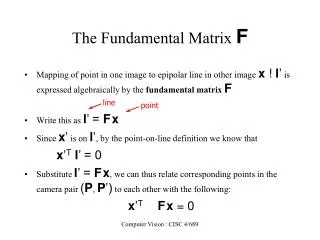
3. Fundamental matrix • The basic description of the projective geometry of two views • The computation of the Fundamental matrix is of utmost theoretical and practical importance (self-calibration method, recovering the 3D projective geometry) • Stage for this chapter • Two views of a scene taken by two (perspective projective) cameras • n (respectively n’) points of interest have been detected in image 1 (respectively in image 2) • Goal: to establish a set of correspondences and to compute the estimate of the Fundamental matrix F that best explains those correspondences

4. Linear methods The key idea:Each point correspondence (m, m') yields one equation , therefore with a sufficient number of point correspondences in general position we can determine F. No knowledge about the cameras or scene structure is necessary. Principle: Let and be two corresponding points. If the Fundamental matrix is , then the epipolar constraint can be rearranged as Where Equation 6.1 is linear and homogeneous in the 9 unknown coefficients of matrix F. Thus if we are given 8 matches, then we will be able, in general, to determine a unique solution for F, defined up to a scale factor. This approach is known as the eight-point algorithm. (6.1)

5. LM: Least-squares solution In this case, we have more linear equations than unknowns, and, in the presence of noise, we look for the minimum of the error criterion which is equivalent to finding the minimum of (6.3) Where 2 solutions 1) closed-form solution via the linear equations 2) solution of subject to

6. LM: Least-squares solution Closed-form solution via the linear equations: One of the coefficients of F is set to 1, yielding a parameterization of F by eight values, which are the ratios of the eight other coefficients to the normalizing one. Let us assume for the sake of discussion that the normalizing coefficient is F33. We can rewrite (6.3) as where is formed with the first 8 columns of , and bis the ninth column of . The solution is known to be if the matrix is invertible. The second method solves the classical problem with The solution is the eigenvector associated with the smallest eigenvalue of .

7. Linear methods: Discussion • The advantage of the eight-point algorithm is that it leads to a noniterative • computation method which is easy to implement using any linear algebra • numerical package; however, we have found that it is quite sensitive to noise, even with numerous data points. • The constraint det(F) = 0 is not satisfied • The quantity that is minimized in (6.2) does not have a good geometric interpretation, one could say that one might be trying to minimize an irrelevant quantity • In all of the linear estimation techniques that will be described in this section, we • deal with projective coordinates of the pixels. In a typical image of dimensions • 512 x 512, a typical image point will have projective coordinates whose orders of • magnitude are given componentwise by the triple (250,250,1). The fact that the • first two coordinates are more than one order of magnitude larger than the third • one has the effect of causing poor numerical conditioning. Solution: normalizing the points in the two images so that their three projective coordinates are of roughly the same order.

8. LM: Enforcing the rank constraint Two-step approximate linear determination of parameters: The idea is to note that in Equation 5.10 of Proposition 5.12, if the epipoles are known, then the Fundamental matrix is a linear function of the coefficients (a,b, c, d) of the epipolar homography. 1. We determine the epipole eby solving the constrained minimization problem subject to , which yields eas the unit norm eigenvector of matrix corresponding to the smallest eigenvalue 2. Once the epipoles are known, we can use Equation 5.10 or, if the epipoles are not at infinity, Equation 5.14, and write the expression as a linear expression of the coefficients of the epipolar homography: where(respectively )are the affine coordinates of (respectively ) This equation can be used to solve for the coefficients of the epipolar homography in a least-squares formulation, thereby completing the determination of the parameters of F.

9. LM: Enforcing the rank constraint Using the closest rank 2 matrix: The matrix Ffound by the eight-point algorithm is replaced by the singular matrix that minimizes the Frobenius norm llF - F'll. This step can be done using a singular value decomposition. If , with , then . Solving a cubic equation: One selects two components of F, say, without loss of generality, F32and F33and rewrites (6.3) as The vector h is made of the first 7 components of the vector f,the matrix is made of the first 7 columns of matrix , and the vectors W8and W9 are the eighth and ninth column vectors of that matrix, respectively. The solution h is We have a linear family of solutions parametrized by F32 and F33.In that family of solutions, there are some that satisfy the condition det(F) = 0. They are obtained by expressing the determinant of the solutions as a function of F32 and F33. One obtains a homogeneous polynomial of degree 3 which must be zero. Solving for one of the two ratios F32 : F33 or F33 : F32 one obtains at least one real solution for the ratio and therefore at least one solution for the Fundamental matrix.

10. Nonlinear methods The distance to epipolar lines The idea is to use a non-quadratic error function and to minimize However, two images should play the symmetric roles It can be written using the fact that .It can be observed that this criterion does not depend on the scale factor used to compute F. The Gradient criterion and an interpretation as a distance Uses criterion

11. Nonlinear methods The “optimal” method The nonlinear method based on the minimization of distances between observed points and reprojected ones where f is a vector of parameters for F, {Mi} are the 3D coordinates of the points in space, and P(f), P’(f) are the perspective projection matrices in the first and second images, given the Fundamental matrix F(f). That is, we estimate not only F, but also the most likely true positions . Because of the epipolar constraint, there are 4 - 1 degrees of freedom for each point correspondence, so the total number of parameters is 3p + 7. The estimation of the Fundamental matrix parameters f can be decoupled from the estimation of the parameters Mi :Since the optimal parameters can be determined from the parameters f,we have to minimize only over f. At each iteration, we have to perform the projective reconstruction of p points. The problem can be rewritten as

12. M-Estimator Let be the residual of the i-thdatum. For example, in the case of the linear methods , in the case of the nonlinear methods The standard least-squares method tries to minimize , which is unstable if there are outliers present in the data. The M-estimators try to reduce the effect of outliers by replacing the squared residuals by another function of the residuals, yielding the error function where p is a symmetric, positive function with a unique minimum at zero and is chosen to be growing slower than the square function. The M-estimator of f based on the function is a vector f which is a solution of the system of qequations (6.16) where the derivative is called the influence function. If we now define define a weight function then Equation 6.16 becomes

13. M-Estimator with the Tukey function otherwise where is some estimated standard deviation of errors and c = 4.6851 is the tuning constant. The corresponding weight function is otherwise

14. Monte Carlo - Least-median-of-squares method It estimates the parameters by solving the nonlinear minimization problem Given ppoint correspondences ,we proceed through the following steps 1) A Monte Carlo type technique is used to draw m random subsamples of q= 7 different point correspondences 2) For each subsample, indexed by J, we use the technique described in Proposition 5.14 to compute the Fundamental matrix FJ.We may have at most 3 solutions 3) Compute the median, denoted by MJ, of the squared residuals 4) Retain the estimate FJfor which MJ is minimal among all m MJ’s

15. Example of estimation with comparison • Pair of calibrated stereo images • There are 241 point matches which are established automatically • Outliers have been discarded • The calibrated parameters of the cameras are not used, but the Fundamental • matrix computed from these parameters serves as a ground truth (+ each F is normalized by its Frobenius norm) e, e’ positions of 2 epipoles RMS = squared distances between points and their epipolar lines CPU = approximate CPU time in seconds when the program is run on a Sparc 20 workstation

16. Better comparison method • Choose randomly a point m in the first image • Draw epipolar line of m in the second image using F1 • If the epipolar line does not intersect the second image, then go to Step 1 • Choose randomly a point m’ on the epipolar line. Note that m and m’ correspond to each other exactly with respect to F1 • Draw the epipolar line of m in the second image using F2 , and compute the distance, denoted by d’1 , between point m’ and line F2m • Draw the epipolar line of m’ in the first image using F2 , and compute the distance, denoted by d1 , between point m and line F2Tm’ • Conduct the same procedure from Step 2 through Step 6, but reversing the roles of F1 and F2, and compute d2 and d’2 • Repeat Step 1 through Step 7 N times • Compute the average distance of d’s, which is the measure of difference between the two Fundamental matrices

17. New comparason • Linear method is very bad • The linear method with prior data normalization gives quite a reasonable result • The nonlinear method based on point-line distances and that based on gradient-weighted epipolar errors give very similar result to those obtained based on minimization of distances between observed points and reprojected ones. The latter should be avoided because it is too time consuming. • M-Estimators or the LMedS method give still better results because they try to limit or eliminate the effect of poorly localized points. The epipolar geometry estimated by LMedS is closer to the one computed through stereo calibration.