Download
1 / 26
260 likes | 382 Views
CFD modeling of large scale LH2 spills in open environment Dr. A.G Venetsanos 1 Prof. J.G. Bartzis 2 1 Environmental Research Laboratory Institute of Nuclear Technology and Radiation Protection National Center for Scientific Research Demokritos Athens, Greece

E N D
CFD modeling of large scale LH2 spills in open environment Dr. A.G Venetsanos1 Prof. J.G. Bartzis2 1Environmental Research Laboratory Institute of Nuclear Technology and Radiation Protection National Center for Scientific Research Demokritos Athens, Greece 2University of Western Macedonia, Kozani, Greece venets@ipta.demokritos.gr
Scope To increase our understanding and predictive ability of LH2 release and dispersion Framework Work performed in the framework of the SBEP activity of HYSAFE NoE Also continuation of previous work (Statharas et al., 2000) Focus NASA-6 large scale LH2 release in open environment, (Witcofski and Chirivella, 1984) ADREA-HF CFD code (inhouse, commercial) extensively applied during the EIHP and EIHP-2 EC funded projects Parametric study performed to investigate the effects of the source model the presence of the elevated pond sides around the source the contact heat transfer between ground and nearby ambient air. Introduction
NASA-6 experimental description Deployment of instrumentation towers and typical instrumentation array Liquid hydrogen spill-line, valve, pond and diffuser 5.11 m3 LH2 released in 38s, mass flow rate 9.5 kg s-1 2.2 m s-1 wind speed at 10m height, 15 ºC ambient temperature and 29% relative humidity
NASA-6 experiment results Temperature deduced concentrations Experiment, t = 20.94 s Experiment, t = 21.33 s
Mean flow equations Mixture mass (fully compressible) Mixture momentum (3 equations) Mixture enthalpy Hydrogen mass fraction (1 equation for liquid + vapour) Turbulence modeling Standard k- model (Launder B. E. and Spalding, 1974) Buoyancy effects included Physics Liquid phase obtained from the equilibrium phase change model Temperature obtained for given enthalpy, pressure and hydrogen mass fraction Ground heat transfer modelled by solving a transient one dimensional energy (temperature) equation inside the ground, with or without contact heat transfer Source modelled as a two phase jet or as pool Earthen sides of pond modelled as a thin fence or not modelled ADREA-HF Modeling strategy
ADREA-HF mean flow equations Mixture mass Mixture momentum Mixture enthaply Hydrogen mass fraction
ADREA-HF standard k- turbulence model Turbulent kinetic energy Dissipation rate of turbulent kinetic energy Eddy viscosity
Two phase jet: Horizontal surface (representing the diffuser): size 0.5x0.5 m2 pointing downwards placed in the first cell next to ground Boundary conditions: vertical velocity -11.47 m s-1 from time 0 to 38 seconds pressure 101325.0 Pa temperature 20.4 K (boiling) void fraction (vapour volume/total volume) 97%. These conditions give: hydrogen liquid mass fraction (liquid mass/total mass) 65% hydrogen density 3.315 kg m-3 hydrogen flow rate equal to 9.5 kg s-1 ADREA-HF source models
Pool: A horizontal open area source (representing the pool) radius 4.45 m constant pointing upwards assumed in place of the ground Boundary conditions on this surface: vertical velocity 0.2535 m s-1 from time 0 to 38 seconds pressure 101325.0 Pa temperature 20.4 K (boiling) void fraction (vapour volume/total volume) 100%. These conditions give hydrogen density 1.207 kg m-3 hydrogen flow rate equal to 9.5 kg s-1 ADREA-HF source models
ADREA-HF ground heat transfer model Energy equation solved inside ground Ground heat flux Contact heat transfer coefficient (Zilitinkevich, 1970) Friction velocity
Phase change criterion: Liquid phase of component-1 appears instantaneously (condensation occurs), when the component-1 mass-fraction exceeds its saturation value in the mixture (Vice versa for evaporation) Distribution into phases: The amount of component-1 in liquid phase is such that a saturation state exists in the gaseous region: ADREA-HF equilibrium phase change model Mass fractions Mixture density
ADREA-HF thin obstacle model Additional resistance forces in the horizontal momentum equations (Andronopoulos et al., 1994)
Domain and grid (Cartesian) X-Z symmetry assumed Domain 175x80x68 m. Computational cells 39600 minimum horizontal cell size 0.6 m close to the source maximum horizontal cell size nearly 10 m close to the domain boundaries minimum vertical cell size 0.2 m near the ground and source maximum vertical cell size about 9 m near the top of domain Discretization Control volume approach Fully implicit formulation First order in time Upwind scheme for convective terms Automatic time step selection (0.001-0.25s) Three step solution sequence One dimensional (in the z-direction) calculation of the approaching boundary layer Three dimensional steady state calculation of the flow over the fence Transient hydrogen release ADREA-HF Solution strategy
ADREA-HF Case 1 predictions versus experiment Jet, with fence, with contact heat transfer Predicted contours of hydrogen concentration (by vol.) on symmetry plane at t = 21 s Experiment, t = 21.33 s
ADREA-HF Case 2 predictions versus experiment Jet, with fence, without contact heat transfer Predicted contours of hydrogen concentration (by vol.) on symmetry plane at t = 21 s Experiment, t = 21.33 s
ADREA-HF Case 3 predictions versus experiment Jet, without fence, with contact heat transfer Predicted contours of hydrogen concentration (by vol.) on symmetry plane at t = 21 s Experiment, t = 21.33 s
ADREA-HF Case 4 predictions versus experiment Pool, without fence, with contact heat transfer Predicted contours of hydrogen concentration (by vol.) on symmetry plane at t = 21 s Experiment, t = 21.33 s
ADREA-HF Case 5 predictions versus experiment Pool, with fence, with contact heat transfer Predicted contours of hydrogen concentration (by vol.) on symmetry plane at t = 21 s Experiment, t = 21.33 s
ADREA-HF Case 1 predictions versus experiment LAuV post calculation The shaded area corresponds to the range of measurements (taken from Verfondern and Dienhart (1997))
The ADREA-HF CFD code was successfully applied to simulate the NASA trial-6 experiment. A series of CFD runs were performed to investigate on the effects of source model, fence presence and contact heat transfer. In all cases considered it was not able to reproduce neither the very sudden changes in cloud structure observed experimentally nor the high levels of concentrations measured at tower 7, located 33.8 m downwind and 12.9 m laterally from the source. This behaviour was attributed to wind meandering, observed during the experiments, but not modelled herein. Entirely different cloud structures were obtained depending on the method the source was modelled. Modelling the source as a two-phase jet, pointing downwards resulted in predicted concentrations in much better agreement with the experiments. Modelling the source as a pool resulted in overestimation of concentration levels. The earthen sides of the pond were modelled as a fence of infinitesimal thickness. The calculations showed that near ground concentration levels downstream the source increased when the fence was removed. This effect was more pronounced when the source was modelled as a jet. Conclusions
Accounting for the temperature difference between ground and adjacent air at the level of the roughness length was found to be very important Using a two-phase jet pointing down, contact heat transfer and including the fence results were the closest to the experimental. Still, the predicted concentration levels on tower 5, 9.4 m are underestimated and at 1 m overestimated suggesting that the predicted cloud is less lifted from ground than in the experiment. This suggests that probably a more intense heat flux from the ground would be required to obtain a better agreement with the experiment. Conclusions