Download
1 / 20
200 likes | 220 Views
Understand linear regression, correlation, and least squares method. Examples and applications in statistical analysis. Practical tips for data modeling.

E N D
Lecture 6: Linear Regression and Correlation Nigel Rozario, MS Jie Zhou, MS H. James Norton, PhD 10/17/2013
Example Points on this line; (0,2) (1,7) (2, 12)
Linear Regression • Linear Regression is an approach to modeling the relationship between a scalar variable y and one or more variables denoted X. • Linear regression has many practical uses. - Prediction, forecasting - quantify the strength of the relationship between y and the Xj
Assumptions • L: Linear (in parameters) • I: Independent • N: Normality • E: The variances of are equal • X: - The regressorsxi are assumed to be error-free, that is they are not contaminated with measurement errors.
CorrelationPearson’s product moment correlation coefficient • Assumptions: x and y values follows bivariate normal For ordinal data not normally distributed, use Spearman’s Correlation
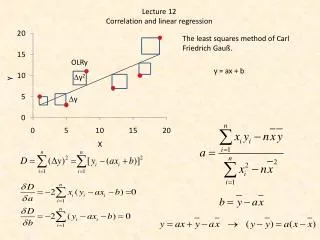
Method of Least Squares • Let’s use an example.. Revised SAT ranking UNC-Chapel Hill Journalism Professor Phil Meyer used statistical techniques (least-square regression) to adjust for different SAT participation rates for the 50 states and the District of Columbia. In essence, the technique adjusts the data to reflect what the SAT scores would likely be if the same percentage of students in all states took the tests.
Outcome variable (Y) This is the p-value of the model. It tests whether R2 is different from 0. Root mean squared error, is the SD of the regression. The closer to zero better the fit. R2 shows the amount of variance of Y explained by X. Two-tail P-value test the hypothesis that each coefficient is different from 0 Expected Score = 1020.61-220.51*Taking_Test Predictor variable (X)
Expected Score (North Carolina) = 1020.61-220.51x(Taking_Test) = 1020.61-220.51x(0.57) = 894.9193 • Residual (or error) = Raw Score – Expected Score = 844 - 894.9193 ≈ -50.9193 Percentage of students who took the test only partly explains what’s the SAT score for each state
Expected sbp = 105.60 + 0.78 x (age)when age = 30, expected sbp = 105.60 + 0.78 x (30) = 129Residual = observed sbp – expected sbp = 137- 129 = 8
Multiple Linear Regression Data (First 10 observations) R2 shows the amount of variance of SBP explained by Age & BMI Two-tail P-value test the hypothesis that each coefficient is different from 0 Reference: Biostatistics: A guide to design, analysis and discovery, 2nd ed [Forthofer, Lee, Hernandez]
Predicted SBP=76.08 + 0.33xAge + 1.3xBMI When Age=28 and BMI=24.33 Predicted SBP=76.08 + 0.33x(28) + 1.3x(24.33) =76.08 + 9.24 + 31.63 = 116.95 Residual = Predicted SBP - Observed SBP = 116.95 – 111 = 5.95
Conclusion • Simple Linear Regression: one covariate x • Multivariate Linear Regression : multiple covariates X • For the previous first example, other factors might influence the SAT scores : - Percentage of parents have college education - The cost on education per student for each state • Adding more covariates, R2 always goes up. This brings up another statistics topic - Goodness of Fit test (GOF)
Questions or Comments? Questions or Comments?