Download
1 / 28
280 likes | 330 Views
Explore the principles of Dynamic Causal Modelling (DCM) for functional MRI connectivity analysis. Learn about Bayesian parameter estimation, statistical inference, neural dynamics, and effective connectivity modeling.

E N D
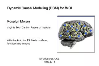
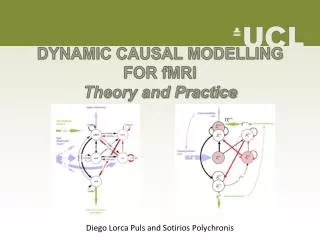
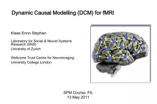
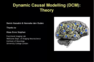
Dynamic Causal Modelling (DCM): Theory Demis Hassabis & Hanneke den Ouden Thanks to Klaas Enno Stephan Functional Imaging Lab Wellcome Dept. of Imaging Neuroscience Institute of Neurology University College London
Overview • Classical approaches to functional & effective connectivity • Generic concepts of system analysis • DCM for fMRI: • Neural dynamics and hemodynamics • Bayesian parameter estimation • Interpretation of parameters • Statistical inference • Bayesian model selection
System analyses in functional neuroimaging Functional specialisation Analyses of regionally specific effects: which areas constitute a neuronal system? Functional integration Analyses of inter-regional effects: what are the interactions between the elements of a given neuronal system? Functional connectivity = the temporal correlation between spatially remote neurophysiological events Effective connectivity = the influence that the elements of a neuronal system exert over another MECHANISM-FREE MECHANISTIC
Models of effective connectivity • Structural Equation Modelling (SEM) • Psycho-physiological interactions (PPI) • Multivariate autoregressive models (MAR)& Granger causality techniques • Kalman filtering • Volterra series • Dynamic Causal Modelling (DCM) Friston et al., NeuroImage 2003
Overview • Classical approaches to functional & effective connectivity • Generic concepts of system analysis • DCM for fMRI: • Neural dynamics and hemodynamics • Bayesian parameter estimation • Interpretation of parameters • Statistical inference • Bayesian model selection
Models of effective connectivity = system models.But what precisely is a system? • System = set of elements which interact in a spatially and temporally specific fashion. • System dynamics = change of state vector in time • Causal effects in the system: • interactions between elements • external inputs u • System parameters :specify the nature of the interactions • general state equation for non-autonomous systems overall system staterepresented by state variables change ofstate vectorin time
LG left FG right LG right FG left Example: linear dynamic system LG = lingual gyrus FG = fusiform gyrus Visual input in the - left (LVF) - right (RVF)visual field. z4 z3 z1 z2 RVF LVF u2 u1 systemstate input parameters state changes effective connectivity externalinputs
z4 z3 z1 z2 CONTEXT RVF LVF u2 u3 u1 LG left FG right LG right FG left Extension: bilinear dynamic system
Bilinear state equation in DCM modulation of connectivity systemstate direct inputs state changes intrinsic connectivity m externalinputs
Overview • Classical approaches to functional & effective connectivity • Generic concepts of system analysis • DCM for fMRI: • Neural dynamics and hemodynamics • Bayesian parameter estimation • Interpretation of parameters • Statistical inference • Bayesian model selection
z λ y DCM for fMRI: the basic idea • Using a bilinear state equation, a cognitive system is modelled at its underlying neuronal level (which is not directly accessible for fMRI). • The modelled neuronal dynamics (z) is transformed into area-specific BOLD signals (y) by a hemodynamic forward model (λ). The aim of DCM is to estimate parameters at the neuronal level such that the modelled BOLD signals are maximally similar to the experimentally measured BOLD signals.
z λ y Conceptual overview Neural state equation The bilinear model effective connectivity modulation of connectivity Input u(t) direct inputs c1 b23 integration neuronal states a12 activity z2(t) activity z3(t) activity z1(t) hemodynamic model y y y BOLD Friston et al. 2003,NeuroImage
u 1 u 2 Z 1 Z 2 Example: generated neural data u1 u2 stimuli u1 context u2 - z1 + - Z1 z2 + + Z2 - -
The hemodynamic “Balloon” model • 5 hemodynamic parameters: important for model fitting, but of no interest for statistical inference • Empirically determineda priori distributions. • Computed separately for each area (like the neural parameters).
LG left LG right FG right FG left Example: modelled BOLD signal Underlying model(modulatory inputs not shown) left LG right LG RVF LVF LG = lingual gyrus Visual input in the FG = fusiform gyrus - left (LVF) - right (RVF) visual field. blue: observed BOLD signal red: modelled BOLD signal (DCM)
Overview • Classical approaches to functional & effective connectivity • Generic concepts of system analysis • DCM for fMRI: • Neural dynamics and hemodynamics • Bayesian parameter estimation • Interpretation of parameters • Statistical inference • Bayesian model selection
Bayes Theorem posterior likelihood ∙ prior Bayesian rule in DCM • Likelihood derived from error and confounds (eg. drift) • Priors – empirical (haemodynamic parameters) and non-empirical (eg. shrinkage priors, temporal scaling) • Posterior probability for each effect calculated and probability that it exceeds a set threshold expressed as a percentage
ηθ|y stimulus function u Parameter estimation in DCM neural state equation • Combining the neural and hemodynamic states gives the complete forward model. • An observation model includes measurement errore and confounds X (e.g. drift). • Bayesian parameter estimation: minimise difference between data and model • Result:Gaussian a posteriori parameter distributions, characterised by mean ηθ|y and covariance Cθ|y. parameters hidden states state equation observation model modelled BOLD response
Overview • Classical approaches to functional & effective connectivity • Generic concepts of system analysis • DCM for fMRI: • Neural dynamics and hemodynamics • Bayesian parameter estimation • Interpretation of parameters • Statistical inference • Bayesian model selection
z4 z3 z1 z2 CONTEXT RVF LVF u2 u3 u1 LG left FG right LG right FG left DCM parameters:interpretation & inference - DCM gives gaussian posterior densities of parameters (intrinsic connectivity, effective connectivity and inputs) Hypothesis: modulation by context > 0 • How can we make inference about effects represented by these parameters • At a single subject level? • At a group level? • How do we select between different models?
ηθ|y Bayesian single-subject analysis • Assumption: posterior distribution of the parameters is gaussian • Use of the cumulative normal distribution to test the probability by which a certain parameter (or contrast of parameters cT ηθ|y) is above a chosen threshold γ: • γ can be chosen as zero ("does the effect exist?") or as a function of the expected half life τ of the neural process: γ= ln 2 / τ ηθ|y Probability
Group analysis • In analogy to “random effects” analyses in SPM, 2nd level analyses can be applied to DCM parameters: Separate fitting of identical models for each subject Selection of bilinear parameters of interest one-sample t-test:parameter > 0 ? paired t-test:parameter 1 > parameter 2 ? rmANOVA:e.g. in case of multiple sessions per subject
Model comparison and selection Given competing hypotheses on structure & functional mechanisms of a system, which model is the best? Which model represents thebest balance between model fit and model complexity? For which model i does p(y|mi) become maximal? Pitt & Miyung (2002), TICS
Bayes theorem: Model evidence: The log model evidence can be represented as: Bayes factor: Bayesian Model Selection Penny et al. 2004, NeuroImage
Hypothesis abouta neural system The DCM cycle Statistical test on parameters of optimal model Definition of DCMs as systemmodels Bayesian modelselection of optimal DCM Design a study thatallows to investigatethat system Parameter estimationfor all DCMs considered Data acquisition Extraction of time seriesfrom SPMs
Inference about DCM parameters: Bayesian fixed-effects group analysis Because the likelihood distributions from different subjects are independent, one can combine their posterior densities by using the posterior of one subject as the prior for the next: Under Gaussian assumptions this is easy to compute: group posterior covariance individual posterior covariances group posterior mean individual posterior covariances and means See: spm_dcm_average.m Neumann & Lohmann, NeuroImage 2003
Laplace approximation: Akaike information criterion (AIC): Bayesian information criterion (BIC): Approximations to model evidence Unfortunately, the complexity term depends on the prior density, which is determined individually for each model to ensure stability. Therefore, we need other approximations to the model evidence. Penny et al. 2004, NeuroImage
DCM parameters = rate constants Integration of a first order linear differential equation gives an exponential function: The coupling parameter athus describes the speed ofthe exponential growth/decay: The coupling parameter a is inversely proportional to the half life of z(t):