Download

1 / 43
460 likes | 705 Views
Explore communication-based models of watermarking in multimedia security, including cryptographic secure transmission, spread spectrum communication, and watermarking schemes. Learn about watermark encoding/decoding, geometric representations, and distribution of unwatermarked works in media and marking spaces. Gain insights into watermark detection, system analysis, and regions of acceptable fidelity.

E N D
Models of Watermarking《 Digital Watermarking: Principles & Practice》 Chapter 3 Multimedia Security
Outline • Communication-based models of watermarking • Geometric models of watermarking • Modeling watermark detection by correlation
Noise n Input message Channel encoder Channel decoder Output message m mn x y Components of Communication Systems • m: the message we want to transmit • x: the codeword encoded by the channel encoder • n: the additive random noise • y: the received signal • mn: the received message A many-to-one function Source coder + modulator
Noise n Channel encoder Channel decoder Output message Encryptor Decryptor m x y mn Decryption key Encryption key Secure Transmission • Cryptography • Prior to transmission, cryptography is used to encrypt a message using a key. • The encrypted message (ciphertext) is transmitted over the channel • At the receiver, the ciphertext is received and decrypted using the related key to reveal the cleartext • Spread Spectrum Communication • Against signal jamming • Modulation is done according to a secret code, which spreads the signal over a wider bandwidth than required Input message
Noise n Input message Output message Watermark encoder Watermark decoder wa wn m cw cwn mn co co Original cover work Watermark key Original cover work Watermark key Noise n Input message Output message Watermark encoder Watermark decoder m wa cw cwn mn Original cover work Watermark key Watermark key Watermarking as Communication Systems Informed Blind
Noise n Input message Output message Watermark encoder Watermark decoder m wa cwn mn cw Watermark key Watermark key Original cover work Watermarking as Comm. with Side Information
A Simple Watermarking Scheme • Embedding • An one-bit message m is embedded. • wr is the predefined reference pattern • The message pattern wm is equal to wr or -wr according to the value of m. • The value controls the trade-off between visibility and robustness • Detection • The linear correlation between the received image c and the reference pattern wr is computed. • Whether a watermark is presented is decided by placing a threshold
Media Space • Watermarking algorithms can be conceptualized in geometric terms • Media space • To view a watermark system geometrically, please imagine a high-dimensional space in which each point representing one Work • Works are thought of as points in a N-dimensional media space • The dimensionality of a media space, N, is the number of samples used to represent each Work • For monochrome images, N is the number of pixels • For RGB images, N is 3*the number of pixels • For continuous and temporal content, such as audio and video, N is the number of samples in the fixed segment in which the watermark is embedded • Each sample is quantized and bounded • Implying a finite but huge set of possible Works, arranged in a rectilinear lattice in media space *
Marking Space • Marking space • Projections or distortions of media space • To analyze systems using more sophisticated algorithms • A watermarking system can be viewed in terms of various regions and probability distributions in media or marking spaces Frequency transform, filtering, block averaging, feature extraction… Determine whether the extracted mark contains a watermark and decode it Simple watermark detector Watermark message Watermark extractor Watermarked Work Vector in marking space Vector in media space
Viewing Geometrically… • Distribution of unwatermarked Works • Describing how likely each Work is • Region of acceptable fidelity • A region in which all Works appear essentially identical to a given cover Work • Detection region • Describing the behavior of the detection algorithm • Embedding distribution/region • Describing the effects of an embedding algorithm • Distortion region • Indicating how Works are likely to be distorted during normal usage
Distribution of Unwatermarked Works • Different works have different likelihoods of entering into a watermark embedder or a detector • In audio, watermarks are more likely to be embedded into music than into pure static • In video, watermarks are more likely to be embedded in images of scenes than in video “snow” • When grasping the properties of a watermarking system, it is important to model the a priori distribution of content we expect the system to process • Gaussian distribution • Laplacian or generalized Gaussian distribution • Result of random, parametric processes • The most important thing • The distribution of unwatermarked content is application dependent • Accuracy of performance estimation relies on correct choices of distributions of Works
Region of Acceptable Fidelity • We can imagine a region around an original image co in which every vector corresponds to an image that is indistinguishable from co • It is VERY DIFFICULT to identify the true region of acceptable fidelity around a given Work, since too little is known about human perception • Approximations by setting a threshold on some measure of perceptual distance • DMSE= Σ (c1[i]-c2[i])2 / Nwhere c1 and c2 are N-vectors in media space. If a limit τMSE is set on this function, the region of acceptable fidelity becomes an N-dimensional ball of radius sqrt(NτMSE ) • DSNR=Σ (c2[i]- c1 [i])2 / Σ c1[i]2 (notice the asymmetry) • Just noticeable difference (JND)
Detection Region • The detection region for a given image and a watermark key is the set of Works in media space that will be decoded by the detector as containing that message • Like the region of acceptable fidelity, the detection region is often defined by a threshold on a measure of the similarity between the detector’s input and a pattern that representing the watermark • Detection measure • Linear correlation: Zlc(c, wr)=c▪wr/N=k|c| cos • Orthogonal projection of of the N-vector c onto the N-vector wr • The set of all points for which this value is greater than the threshold is the set of all points on one side of a plane perpendicular to wr.
Detection region Region of acceptable fidelity Points in the intersection represent successfully watermarked versions of co Illustrating Regions in the Media Space • All points within the circular region of acceptable fidelity and to the right of the planar edge of the detection region corresponds to versions of co that are within an acceptable range of fidelity and that will cause the detector to report the presence of the watermark cwn cw co wr
Detection region wr Embedding Distribution or Region • A watermark embedder is a function that maps a Work, a message, and possibly a key into a new Work • It is generally a deterministic function • Embedding distribution • Since the original Work can be viewed as drawn randomly from the distribution of unwatermarked Works, the probability that a given Work will be output by the embedder is just the probability that a Work leads to it, C0 is drawn from the distribution of unwatermarked Works • Some embedding algorithms define an embedding distribution in which every point has a non-zero probability • Even images outside the detection region can be arrived by applying the embedding algorithms into some other images There is some non-zero probability that a Work outside the detection area will be outputted
Detection region wr Improving The Prescribed Algorithm • By exploiting the side information, an 100% embedding effectiveness can be guaranteed (the embedding region is completely contained in the detection region) The vector added to each unwatermarked Work is chosen to guarantee that the resulting work lies in detection region
Distortion Region • To judge the effects of attacks, we need to know the probability p(cwn|cw) – the distortion distribution • This conditional probability is exactly the same type of distribution used to characterize transmission channels in traditional communication theory • Theoretical discussions begins with the assumption that the distortion distribution can be modeled as additive Gaussian noise • Simplified, not close to reality • Few distortions are even random, most are in general deterministic functions • The noise added is highly dependent on the content • E. g. cropping • Distortion distribution is multi-modal, unlikely to be produced by a Gaussian noise process.
Linear Correlation • The linear correlation between two vectors is the average product of their elements. • The detection region consists of all points on one side of a hyperplane. • The hyperplane is perpendicular to the reference mark, and its distance from the origin is determined by the detection threshold • Robustness concerns • In high dimensions, vectors drawn from Gaussian distribution tend to be nearly orthogonal to a given reference mark • A Gaussian noise attacked vector tends to be parallel to the edge Detection region wr
Normalized Correlation • The extracted mark and the reference mark are normalized to unit magnitude before computing the inner product between them wr Detection region • Lower threshold leads to wider cone • Equivalent scheme:
a a’ b b’ Correlation Coefficient • The means of two vectors are subtracted out before computing the normalized correlation • The result of the subtraction is a vector that is orthogonal to the diagonal. • The resulting vector lies in an (N-1)-space that is orthogonal to the diagonal of the N-dimensional coordinate system
Algorithm 1: Blind Embedding and Linear Correlation Detection E_Blind/D_LC: single reference pattern: if (with watermark)
Assume and n are drawn from Gaussian distributions, and that is, if (without watermark) The D_LC detector outputs
Hypothesis Testing The is selected based on the resulting false positive probability (a major concern for watermarking applications) False Alarm probability (Area of the shaded region)
Algorithm 2: E_Fixed_Lc / D_LC In the E_Blind embedder, we assume is small. In E_Fixed_LC system, we do not make this assumption. Instead, we set to explicitly account for the effects of this inherent correlation. Set (still assume β:embedding strength parameter
By substituting for and solving for we obtain After computing the rest of the E_Fixed_LC algorithm proceeds the same way as the E_Blind algorithm.
Algorithm 3: Block-based, Blind Embedding and Correlation Coefficient Detection In this system, we extract watermarks by averaging blocks of an image. This results in a 64-dimensional marking space. Watermarks are embedded in marking space by simple, blind embedding and the resulting changes are projected back to the full size.
E_Blk_Blind / D_Blk_CC D_Blk_CC: To extract a watermark from an image, the image is divided into blocks and all blocks are averaged into one array of 64 values. w:width; h:high; B:no of blocks. To detect a watermark in an extracted mark, the extracted mark is compared against a predefined reference mark. The reference mark in this system is an array of values (i.e., a vector in marking space)
Correlation coefficients differ from linear correlations in two • ways. • Subtract the means of the two vectors before correlating them. • The detection value is unaffected if a constant is added • to all elements of either of the two vectors. • (2) Normalize the linear correlation by the magnitudes of the two vectors. • The detection is unaffected if all elements of either • vector are multiplied by a constant. • A system using the correlation coefficient (CC) is robust to changes in image brightness and contrast.
is the mean value of X CC is the inner product of and after each has been normalized to have unit magnitude.
D_Blk_CC detector outputs where is a constant threshold.
E_Blk_Blind • Extract a mark, from the unwatermarked work • Choose a new vector, in marking space that is close to the extracted mark but is (hopefully) inside the detection region. • Project the new vector back into media space to obtain the watermarked work,
The extraction process in the embedder is the same as that in the detector. Watermarks are embedded in marking space using E_Blind. The resulting vector is projecting back to which is perceptually close to i.e., we simply distribute each element of the desire change in the extracted mark uniformly to all contributing pixels.
If we were to use LC in the detector rather than CC, the performance would be identical to that of E_Blind / D_LC using a reference pattern that consists of a single pattern tiled over the full size of the image, that is
E_Blind/D_LC v.s. E_Blk_Blind / D_Blk_CC • D_Blk_CC: • robust to certain changes in image brightness and contrast. • D_Blk_CC detector is computationally cheaper that the • D_LC detector. • On the other hand, the number of possible reference marks, and hence the watermark key space, for E_Blk_Blind / D_Blk_CC is much smaller that that for E_Blind / D_LC. • Moreover, many of those reference marks lead to poor statistical performance the reference marks must be carefully designed.