Download
1 / 43
430 likes | 434 Views
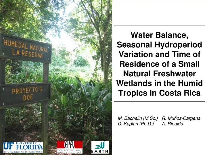
Water Balance, Seasonal Hydroperiod Variation and Time of Residence of a Small Natural Freshwater Wetlands in the Humid Tropics in Costa Rica. M. Bachelin (M.Sc.) R. Mu ñ oz-Carpena D. Kaplan (Ph.D.) A. Rinaldo. Acknowledgments : Funding : UF Gatorade Foundation, Dr. Win Phillips

E N D
Water Balance, Seasonal Hydroperiod Variation and Time of Residence of a Small Natural Freshwater Wetlands in the Humid Tropics in Costa Rica M. Bachelin (M.Sc.) R. Muñoz-Carpena D. Kaplan (Ph.D.) A. Rinaldo
Acknowledgments: Funding: UF Gatorade Foundation, Dr. Win Phillips EARTH cooperators: Warner Rodriguez, Julio Tejada, Faelen Koln and Maria Floridalma Miguel USDA-ARS: Dr. Thomas Potter UF: Paul Lane, Dr. Bin Gao Dr. Timothy G. Townsend, Dr. Hwidong Kim, For more info, contact : carpena@ufl.edu
Outline • Motivation • Part 1 : Field study 1.1 Introduction, motivation and objectives 1.2 Material and methods 1.3 Results: 1.3.1 Water stages 1.3.2 Water budget 1.3.3 Model of the water volume and area 1.3.4 Water quality information 1.3.5 Comparison of the volume 1.4 Conclusions • Summary and Take Home • Part 2 : Tracer study • 2.1 Introduction, motivation and objectives • 2.2 Material and methods • 2.3 Results • 2.3.1 Bromide concentration • 2.3.2 Velocities and preferential chanels • 2.3.3 Br - comparison with SF6 • 2.4 Conclusions
Location of the wetland in EARTH University Campus, Limon province, Costa Rica Nicaragua 1km Costa Rica Location of study wetland area Panama • Collaboration Project: • UF and EARTH University
Why this wetland ? • Tropical natural freshwater wetland • Less studied than temperate ones • Inventory/hydrological studies focused on large systems • Abundance and ubiquitous distribution of small wetlands in the tropics of Central America • Generation of information on hydrology support public decision-making to maintain its sustainability • “La Reserva” wetland • Single regulated outlet • No specific inlet • Small area (9 ha)
1.1 Objectives of the study • Evaluate the spatially and temporally complex and dynamic hydrology of a natural wetland in the humid tropics of the Atlantic region of Costa Rica : • Quantify and analyse the key components in the water balance; • Identify hydroperiod frequency and inter-annual water surface and storage variation during one year of water stages monitoring; • Assess the stability of the hydrologic response of the wetland as an indicator of predominant wet and dry trends through the year and natural water quality function potential.
1.2.1 Instrument location in the wetland • Field work May 2008 • Network of automatic field devices • Surface water tracers (Br-, SF6) • Topographical Survey R. Muñoz-Carpena, D. Kaplan, P. Lane J. Tejada, F. Kolln • Field work May 2009: • New water level station • Topographical Survey • Runoff plots • R. Muñoz-Carpena, P. Lane, M. Bachelin • W. Rodriguez, F. Ros
Water stage recorder • Selection: simplicity, easy maintenance, high accuracy and low cost (Schumann and Muñoz–Carpena, 2002) • Very simple to install and manage (important in harsh field conditions, annual precip.=4500 mm) • All components (potentiometer, pulley, floats and datalogger) inside a PVC pipe • Data logger converts the analog signal from the potentiometer to a digital signal: • Resolution : 0.78 cm per step • Step : every 15 minutes • Water elevation is calculated by knowing the sensor range of the device depending on the effective diameter of the pulley
1.2.2 Water budget • dS = I – O = P + RO – ETP – Q • dS = change in water volume over an interval of time is the difference between the inflow and the outflow • I= Inputs= precipitation (P) and runoff (RO) • O= Outputs= evapotranspiration (ETP) and outflow (Q) • Daily volume [m3]: • P and ETP referred to the most frequent surface water area (1.56 ha) • RO referred to the full catchment area (7.58 ha)
Water budget • Key components: • Precipitation : « isolated » input • Outflow :remained as an important output
1.2.3 Topographical survey • Survey 2008: 183 data points • optical level and compas • Survey 2009: 181 data points • laser andGPS
1.2.4 Model of daily volume and area • Data points from the topographical survey used to generate a high-resolution 3D topographical model of the catchment area • Daily and weekly average of the water stages to generate a water surface grid • - Water surface elevation
1.3.1 Dataset of the field instrumentation • Spatial: • Hydraulic gradient • Stability : branches > main body > outlet Water surface elevation Q
1.3.1 Dataset of the field instrumentation • Temporal: • Variation : noticeable for dry/wet events of successive days (>3)
Q P RO ETP 1.3.2 Water budget • Components : • Inputs: precipitation P and runoff RO • Outputs: evapotranspiration ETP and outflow Q • Storage : • Negative : mostly outflow • Positive : runoff contribution Balance
1.3.3 Daily volume and area (1/5) • Yearly: stability and auto-regulation of the system • Inter-annual: isolated area/storage variation correspond to prolonged wet/dry condition
1.3.3 Comparison of volumes (2/5) • Same trends (ρ =0.463, Vmodel = 0.133*Vbudget + 2.854) • Volumes from water budget have higher isolated peaks : • Outflow submerged • Additional input or output (subsurface flow, leakage, runoff estimation…)
CI95% 1.3.3 Daily volume and area (3/5) • Frequency distribution of the daily water area
1.3.3 Flooding variation(4/5) • Water surfaces representing: • The most frequent flooded area • The lower and upper boundary of the 95% confidence interval of the frequency distribution
1.3.3 Water depth variation(5/5) • Small floodingvariation : • Difference in the 95% confidence interval: 16.5% • Internal variation of water depth, variation of storage • Difference in the 95% confidence interval: 24.2% • Weekly and daily animation…
CI95% 1.3.4 Water quality information • Water time residence in the wetland: Tr = Q / V …
1.3.4 Water quality information • Natural potential of the quality function with k-C* Model (estimated treatment wetland performance, Kadlec and Knight, 1995) : • C2 = C*+(C1-C*)exp(-kA/0.0365Q) • C1 = Inlet concentration [mg/L] • C2 = Outlet concentration [mg/L] • C* = Irreductible background wetland concentation [mg/L] • k = Reduction rate constant [m/yr] • A = Wetland area [m2] • Q = Flow [m3/s] … = IC95%
1.4 Conclusions • System stable and auto-regulated • Small daily variation in flooding frequency and storage • Frequency and duration of the variation in flooded area is not a decisive factor for a vegetation type • Good water quality potential • Water balance can be improved • Driven by precipitation and the outflow • Additional parameters ? • Estimated runoff
2.1 Introduction and objectives • Wetland: natural potential of the water to remove pollutant and improve water quality • Multi-tracer study: • 1. To explore the hydraulic characteristics of the wetland (velocities, pathways, residence time distribution and water mixing); • 2. To assess the feasibility of using Sulfure Hexafluoride as a surface tracer compared to bromide under humid tropical and slow flow conditions.
2.2.1 Preparation, injection and sampling • Field work in 2008: • Tracer preparation in the field • Reference buckets at each site • Injection from opposite branches • Daily sampling (18 sites, 3 weeks)
2.2.2 Sample analysis: SF6 • Sulfur Hexafluoride (SF6): • Non conservative gas • Low solubility in water • Natural low concentration (10-15 M) and detectable in small amount (10-16 M) • Gas chromatograph with electron capture detector (GC/ECD) • Daily calibration curve • Method detection limit: 10-6 • Manual injection and identification
2.2.3 Sample analysis: Br - • Bromide (Br-): • Salt • Conservative and robust • High dilution rate in water • High Pressure Liquid Chromatography (HPLC) with electrochemical detection • Calibration curve before each samples set • Method detection limit: 10-10 • Direct calculation of the peak concentration
2.3.1 Bromide concentration by site (1/2) • Reference buckets: stable [Br-] • Injection sites (6 & 7): quick decrease (until background [Br-])
2.3.1 Bromide concentration by site (2/2) • Low [Br-] with peak tracer cloud passing: • Sites A & 5: One peak • Sites 4, 3 & 2: Two peaks • Site B: edges effect, slow flow and mixing
2.3.2 Velocities and preferential chanels • Velocity estimation [m/day]: • V = distance from injection site / time to peak from injection day • S6: Longer pathway, faster velocities (V central < V edges) • S7: Shorter pathway, slower velocities (V central > V edges)
2.3.3 Br - comparison with SF6 • No significant [SF6] peak, low and fairly stable concentrations • Similar fast decrease of [SF6] from reference bucket and at injection sites: • Too fast volatilization during transport
2.4 Conclusions • Bromide: successful tracer in shallow and slow surface flow in humid and tropical climate • Sulfur Hexafluoride: not adapted to these conditions • Average flow velocities (7-26 m/day) in the same range than velocities calculated with the time residence and the longest path along the wetland (6-11 m/day) • Time to peak and distance between sites gave preliminary analysis to study the hydraulic caracteristics of the wetland (flowpaths, velocities and preferential chanels)
Summary – Take home • The small wetland proved stable and auto-regulated • Small daily variation in flooding frequency and storage • Residence times (20-50 days) obtained for this wetland sindicate good water quality potential with expected removal of common pollutants (BOD, TSS, TN, TP) between 72-98% through the year. • Hydrological and tracer study methods provided consistent average flow velocities (7-26 m/day) in the wetlands through the year. • Time to peak and distance between sites gave preliminary analysis to study the hydraulic caracteristics of the wetland (flowpaths, velocities and preferential chanels) and indicates that the wetland is heterogeneous with fast and slow flow areas. • These findings support the important role that small and ubiquitous wetlands in the humid tropics can play in the environmental quality of these areas
Future steps • Improvement of rainfall/runoff estimates with field plot • Inverse modeling of tracer breakthrough curve
Thank you for your attention ! Questions ?