Download
1 / 53
530 likes | 660 Views
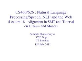
CS460/626 : Natural Language Processing/Speech, NLP and the Web (Lecture 26– Recap HMM; Probabilistic Parsing cntd ). Pushpak Bhattacharyya CSE Dept., IIT Bombay 15 th March, 2011. Formal Definition of PCFG. A PCFG consists of A set of terminals {w k }, k = 1,….,V

E N D
CS460/626 : Natural Language Processing/Speech, NLP and the Web(Lecture 26– Recap HMM; Probabilistic Parsing cntd) Pushpak BhattacharyyaCSE Dept., IIT Bombay 15thMarch, 2011
Formal Definition of PCFG • A PCFG consists of • A set of terminals {wk}, k = 1,….,V {wk} = { child, teddy, bear, played…} • A set of non-terminals {Ni}, i = 1,…,n {Ni} = { NP, VP, DT…} • A designated start symbol N1 • A set of rules {Ni j}, where j is a sequence of terminals & non-terminals NP DT NN • A corresponding set of rule probabilities
Rule Probabilities • Rule probabilities are such that E.g., P( NP DT NN) = 0.2 P( NP NN) = 0.5 P( NP NP PP) = 0.3 • P( NP DT NN) = 0.2 • Means 20 % of the training data parses use the rule NP DT NN
Probabilistic Context Free Grammars • DT the 1.0 • NN gunman 0.5 • NN building 0.5 • VBD sprayed 1.0 • NNS bullets 1.0 • S NP VP 1.0 • NP DT NN 0.5 • NP NNS 0.3 • NP NP PP 0.2 • PP P NP 1.0 • VP VP PP 0.6 • VP VBD NP 0.4
Example Parse t1` S1.0 P (t1) = 1.0 * 0.5 * 1.0 * 0.5 * 0.6 * 0.4 * 1.0 * 0.5 * 1.0 * 0.5 * 1.0 * 1.0 * 0.3 * 1.0 = 0.00225 • The gunman sprayed the building with bullets. NP0.5 VP0.6 NN0.5 DT1.0 PP1.0 VP0.4 P1.0 NP0.3 NP0.5 VBD1.0 The gunman DT1.0 NN0.5 with NNS1.0 sprayed the building bullets
Another Parse t2 S1.0 • The gunman sprayed the building with bullets. P (t2) = 1.0 * 0.5 * 1.0 * 0.5 * 0.4 * 1.0 * 0.2 * 0.5 * 1.0 * 0.5 * 1.0 * 1.0 * 0.3 * 1.0 = 0.0015 NP0.5 VP0.4 NN0.5 DT1.0 VBD1.0 NP0.2 The gunman sprayed NP0.5 PP1.0 DT1.0 NN0.5 P1.0 NP0.3 NNS1.0 the building with bullets
Probability of a sentence Nj NP • Notation : • wab – subsequence wa….wb • Nj dominates wa….wb or yield(Nj) = wa….wb wa……………..wb the..sweet..teddy ..bear • Probability of a sentence = P(w1m) Where t is a parse tree of the sentence If t is a parse tree for the sentence w1m, this will be 1 !!
Assumptions of the PCFG model • Place invariance : P(NP DT NN) is same in locations 1 and 2 • Context-free : P(NP DT NN | anything outside “The child”) = P(NP DT NN) • Ancestor free : At 2, P(NP DT NN|its ancestor is VP) = P(NP DT NN) S NP VP 1 The child NP 2 The toy
Probability of a parse tree • Domination :We say Nj dominates from k to l, symbolized as , if Wk,lis derived from Nj • P (tree |sentence) = P (tree | S1,l ) where S1,l means that the start symbol S dominates the word sequence W1,l • P (t |s) approximately equals joint probability of constituent non-terminals dominating the sentence fragments (next slide)
Probability of a parse tree (cont.) S1,l NP1,2 VP3,l V3,3 PP4,l DT1 N2 w1 w2 P4,4 NP5,l w3 w4 w5 wl P ( t|s ) = P (t | S1,l ) = P ( NP1,2, DT1,1 , w1, N2,2, w2, VP3,l, V3,3 , w3, PP4,l, P4,4 , w4, NP5,l, w5…l |S1,l) = P ( NP1,2 , VP3,l | S1,l) * P ( DT1,1 , N2,2 | NP1,2) * D(w1 | DT1,1) * P (w2 | N2,2) * P (V3,3, PP4,l | VP3,l) * P(w3 | V3,3) * P( P4,4, NP5,l | PP4,l ) * P(w4|P4,4) * P (w5…l | NP5,l) (Using Chain Rule, Context Freeness and Ancestor Freeness )
HMM ↔ PCFG • O observed sequence ↔ w1msentence • X state sequence ↔ t parse tree • model ↔ G grammar • Three fundamental questions
HMM ↔ PCFG • How likely is a certain observation given the model?↔ How likely is a sentence given the grammar? • How to choose a state sequence which best explains the observations?↔ How to choose a parse which best supports the sentence? ↔ ↔
HMM ↔ PCFG • How to choose the model parameters that best explain the observed data? ↔ How to choose rule probabilities which maximize the probabilities of the observed sentences? ↔
HMM Definition • Set of states: S where |S|=N • Start state S0 /*P(S0)=1*/ • Output Alphabet: O where |O|=M • Transition Probabilities: A= {aij} /*state i to state j*/ • Emission Probabilities : B= {bj(ok)} /*prob. of emitting or absorbing ok from state j*/ • Initial State Probabilities: Π={p1,p2,p3,…pN} • Each pi=P(o0=ε,Si|S0)
Markov Processes • Properties • Limited Horizon: Given previous t states, a state i, is independent of preceding 0 to t-k+1 states. • P(Xt=i|Xt-1, Xt-2 ,…X0) = P(Xt=i|Xt-1, Xt-2… Xt-k) • Order k Markov process • Time invariance: (shown for k=1) • P(Xt=i|Xt-1=j) = P(X1=i|X0=j) …= P(Xn=i|Xn-1=j)
Three basic problems (contd.) • Problem 1: Likelihood of a sequence • Forward Procedure • Backward Procedure • Problem 2: Best state sequence • Viterbi Algorithm • Problem 3: Re-estimation • Baum-Welch ( Forward-Backward Algorithm )
Probabilistic Inference • O: Observation Sequence • S: State Sequence • Given O find S* where called Probabilistic Inference • Infer “Hidden” from “Observed” • How is this inference different from logical inference based on propositional or predicate calculus?
Essentials of Hidden Markov Model 1. Markov + Naive Bayes 2. Uses both transition and observation probability 3. Effectively makes Hidden Markov Model a Finite State Machine (FSM) with probability
Probability of Observation Sequence • Without any restriction, • Search space size= |S||O|
Continuing with the Urn example Colored Ball choosing Urn 1 # of Red = 30 # of Green = 50 # of Blue = 20 Urn 3 # of Red =60 # of Green =10 # of Blue = 30 Urn 2 # of Red = 10 # of Green = 40 # of Blue = 50
Example (contd.) Observation/output Probability Transition Probability Given : and Observation : RRGGBRGR What is the corresponding state sequence ?
Diagrammatic representation (1/2) G, 0.5 R, 0.3 B, 0.2 0.3 0.3 0.1 U1 U3 R, 0.6 0.5 0.6 0.2 G, 0.1 B, 0.3 0.4 0.4 R, 0.1 U2 G, 0.4 B, 0.5 0.2
Diagrammatic representation (2/2) R,0.03 G,0.05 B,0.02 R,0.18 G,0.03 B,0.09 R,0.15 G,0.25 B,0.10 R,0.18 G,0.03 B,0.09 U1 U3 R,0.02 G,0.08 B,0.10 R,0.06 G,0.24 B,0.30 R,0.24 G,0.04 B,0.12 R, 0.08 G, 0.20 B, 0.12 U2 R,0.02 G,0.08 B,0.10
Probabilistic FSM (a1:0.3) (a1:0.1) (a2:0.4) (a1:0.3) S1 S2 (a2:0.2) (a1:0.2) (a2:0.2) (a2:0.3) The question here is: “what is the most likely state sequence given the output sequence seen”
Developing the tree a2 a1 € 1.0 0.0 Start 0.3 0.2 0.1 0.3 • . • . 0.3 0.0 1*0.1=0.1 S1 S2 S2 S1 S2 S1 S2 S2 S1 S1 0.0 0.2 0.2 0.4 0.3 • . • . 0.1*0.2=0.02 0.1*0.4=0.04 0.3*0.3=0.09 0.3*0.2=0.06 Choose the winning sequence per state per iteration
Tree structure contd… 0.09 0.06 a2 a1 0.3 0.2 0.1 0.3 • . • . 0.027 0.012 0.018 0.09*0.1=0.009 S2 S1 S1 S2 S2 S2 S1 S1 S1 S2 0.3 0.2 0.4 0.2 • . 0.0048 0.0081 0.0054 0.0024 The problem being addressed by this tree is a1-a2-a1-a2 is the output sequence and μ the model or the machine
Viterbi Algorithm for the Urn problem (first two symbols) S0 ε 0.2 0.5 0.3 U1 U2 U3 0.15 0.02 0.18 0.03 0.18 0.06 R 0.08 0.24 0.02 U1 U2 U3 U1 U2 U3 U1 U2 U3 0.015 0.04 0.075* 0.018 0.006 0.036* 0.048* 0.036 0.006 *: winner sequences
Markov process of order>1 (say 2) • O0O1 O2 O3 O4 O5 O6 O7 O8 • Obs:ε R R G G B R G R • State: S0 S1 S2 S3 S4 S5 S6 S7 S8 S9 Same theory works P(S).P(O|S) = P(O0|S0).P(S1|S0). [P(O1|S1). P(S2|S1S0)]. [P(O2|S2). P(S3|S2S1)]. [P(O3|S3).P(S4|S3S2)]. [P(O4|S4).P(S5|S4S3)]. [P(O5|S5).P(S6|S5S4)]. [P(O6|S6).P(S7|S6S5)]. [P(O7|S7).P(S8|S7S6)]. [P(O8|S8).P(S9|S8S7)]. We introduce the states S0 and S9 as initial and final states respectively. • After S8 the next state is S9 with probability 1, i.e., P(S9|S8S7)=1 O0 is ε-transition
Adjustments • Transition probability table will have tuples on rows and states on columns • Output probability table will remain the same • In the Viterbi tree, the Markov process will take effect from the 3rd input symbol (εRR) • There will be 27 leaves, out of which only 9 will remain • Sequences ending in same tupleswill be compared • Instead of U1, U2 and U3 • U1U1, U1U2, U1U3, U2U1, U2U2,U2U3, U3U1,U3U2,U3U3
Forward probability F(k,i) • Define F(k,i)= Probability of being in state Si having seen o0o1o2…ok • F(k,i)=P(o0o1o2…ok , Si ) • With m as the length of the observed sequence • P(observed sequence)=P(o0o1o2..om) =Σp=0,N P(o0o1o2..om , Sp) =Σp=0,N F(m , p)
Forward probability (contd.) F(k , q) = P(o0o1o2..ok , Sq) = P(o0o1o2..ok , Sq) = P(o0o1o2..ok-1 , ok ,Sq) = Σp=0,N P(o0o1o2..ok-1 , Sp , ok ,Sq) = Σp=0,N P(o0o1o2..ok-1 , Sp ). P(om ,Sq|o0o1o2..ok-1 , Sp) = Σp=0,N F(k-1,p). P(ok ,Sq|Sp) = Σp=0,N F(k-1,p). P(Sp Sq) ok • O0O1O2O3 … Ok Ok+1 … Om-1Om • S0 S1S2 S3 … Sp Sq…SmSfinal
Backward probability B(k,i) • Define B(k,i)= Probability of seeing okok+1ok+2…omgiven that the state was Si • B(k,i)=P(okok+1ok+2…om\ Si ) • With m as the length of the observed sequence • P(observed sequence)=P(o0o1o2..om) = P(o0o1o2..om| S0) =B(0,0)
Backward probability (contd.) B(k , p) = P(okok+1ok+2…om \ Sp) = P(ok+1ok+2…om , ok |Sp) = Σq=0,N P(ok+1ok+2…om , ok , Sq|Sp) = Σq=0,N P(ok ,Sq|Sp) P(ok+1ok+2…om|ok ,Sq ,Sp ) = Σq=0,N P(ok+1ok+2…om|Sq). P(ok , Sq|Sp) = Σq=0,N B(k+1,q). P(Sp Sq) ok • O0O1O2O3 … Ok Ok+1 … Om-1Om • S0 S1S2 S3 … Sp Sq…SmSfinal
Interesting Probabilities N1 What is the probability of having a NP at this position such that it will derive “the building” ? - Inside Probabilities NP The gunman sprayed the building with bullets 1 2 3 4 5 6 7 Outside Probabilities What is the probability of starting from N1 and deriving “The gunman sprayed”, a NP and “with bullets” ? -
Interesting Probabilities • Random variables to be considered • The non-terminal being expanded. E.g., NP • The word-span covered by the non-terminal. E.g., (4,5) refers to words “the building” • While calculating probabilities, consider: • The rule to be used for expansion : E.g., NP DT NN • The probabilities associated with the RHS non-terminals : E.g., DT subtree’s inside/outside probabilities & NN subtree’s inside/outside probabilities
Outside Probability • j(p,q) :The probability of beginning with N1& generating the non-terminal Njpq and all words outside wp..wq N1 Nj w1 ………wp-1 wp…wqwq+1 ………wm
Inside Probabilities • j(p,q) :The probability of generating the words wp..wq starting with the non-terminal Njpq. N1 Nj w1 ………wp-1 wp…wqwq+1 ………wm
Outside & Inside Probabilities: example N1 NP The gunman sprayed the building with bullets 1 2 3 4 5 6 7
Calculating Inside probabilities j(p,q) Base case: • Base case is used for rules which derive the words or terminals directly E.g., Suppose Nj = NN is being considered & NN building is one of the rules with probability 0.5
Induction Step: Assuming Grammar in Chomsky Normal Form Induction step : Nj • Consider different splits of the words - indicated by dE.g., the huge building • Consider different non-terminals to be used in the rule: NP DT NN, NP DT NNS are available options Consider summation over all these. Nr Ns wp wd wd+1 wq Split here for d=2 d=3
The Bottom-Up Approach NP0.5 • The idea of induction • Consider “the gunman” • Base cases : Apply unary rules DT the Prob = 1.0 NN gunman Prob = 0.5 • Induction : Prob that a NP covers these 2 words = P (NP DT NN) * P (DT deriving the word “the”) * P (NN deriving the word “gunman”) = 0.5 * 1.0 * 0.5 = 0.25 DT1.0 NN0.5 The gunman
Parse Triangle • A parse triangle is constructed for calculating j(p,q) • Probability of a sentence using j(p,q):
Parse Triangle • Fill diagonals with
Parse Triangle • Calculate using induction formula
Example Parse t1 S1.0 Rule used here is VP VP PP • The gunman sprayed the building with bullets. NP0.5 VP0.6 NN0.5 DT1.0 PP1.0 VP0.4 P1.0 NP0.3 NP0.5 VBD1.0 The gunman DT1.0 NN0.5 with NNS1.0 sprayed the building bullets
Another Parse t2 S1.0 Rule used here is VP VBD NP • The gunman sprayed the building with bullets. NP0.5 VP0.4 NN0.5 DT1.0 VBD1.0 NP0.2 The gunman sprayed NP0.5 PP1.0 DT1.0 NN0.5 P1.0 NP0.3 the building with NNS1.0 bullets