Download
1 / 57
570 likes | 765 Views
Applying GCMs to terrestrial exoplanets. F.Forget , R. Wordsworth B. Charnay, E. Millour, F. Codron, J.Leconte, F. Selsis * , LMD, Institut Pierre Simon Laplace, Université Pierre et Marie Curie, BP 99, 75005 Paris, France * LAB, (CNRS; Université Bordeaux I).

E N D
Applying GCMs to terrestrial exoplanets F.Forget, R. Wordsworth B. Charnay, E. Millour, F. Codron, J.Leconte, F. Selsis*, LMD, Institut Pierre Simon Laplace, Université Pierre et Marie Curie, BP 99, 75005 Paris, France * LAB, (CNRS; Université Bordeaux I)
Atmospheres in the solar system Triton NEPTUNE Pluto • GIANT PLANETS • Terrestrial atmospheres URANUS Titan SATURNE JUPITER Mars Earth Mercury Venus
MARS TITAN TERRE VENUS • ~a few GCMs • (LMD, Univ. of Chicago, Caltech, Köln…) • Coupled cycles: • Aerosols • Photochemistry • Clouds • Several GCMs • (NASA Ames, Caltech, GFDL, LMD, AOPP, MPS, Japan, York U., Japan, etc…) • Applications: • Dynamics & assimilation • CO2 cycle • dust cycle • water cycle • Photochemistry • thermosphere and ionosphere • isotopes cycles • paleoclimates • etc… • Many GCM teams • Applications: • Weatherforecast • Assimilation and climatology • Climate projections • Paleoclimates • chemistry • Biosphere / hydrospherecryosphere / oceanscoupling • Manyother applications ~1 true GCMs Coupling dynamic & radiative transfer (LMD) 6 GCMs with simplified physics PLUTO 1 full GCM (LMD) TRITON 1 full GCM (LMD)
What we have learned from solar system GCMs • To first order: GCMs work • A few equations can build « planet simulators » with a realistic, complex behaviour and strong prediction capacities • However the devil is in the details: • Problems with • Positive feedbacks and unstability (e.g. sea ice and land ice albedo feedback on the Earth) • Non linear behaviour and threshold effect (e.g. dust storms on Mars) • Complex subgrid scale process and poorly known physics (e.g. clouds on the Earth) • System with extremely long « inertia » with small forcing (e.g. Venus circulation). Sensitivity to intrinsinc dynamical core conserving properties Sensitivity to initial state Need to somewhat « tune » a few model parameters to accurately model an observed planet and predict its behaviour
Mars dynamical core intercomparisons (Mischna and Wilson 2008)
Participating Model Specs Various models provided various combinations of model resolution, damping (α=2, 4) and vertical levels.
Full intercomparison Johnson et al. 2008
The science of Simulating the unknown: From planet GCMs to extrasolar planet GCMs.
How GCM work ? :The minimum General Circulation Model for a terrestrial planet Most processes can be described by equations that we have learned to solve with some accuracy • 1) 3D Hydrodynamical code • to compute large scale atmospheric motions and transport • 2) At every grid point : Physical parameterizations • to force the dynamic • to compute the details of the local climate • Radiative heating & cooling of the atmosphere • Surface thermal balance • Subgrid scale atmospheric motions • Turbulence in the boundary layerConvection Relief drag Gravity wave drag • Specific process : ice condensation, cloud microphysics, etc…
Toward a “generic” Global climate model (LMD) • Use “universal” parametrisations for all planets: • Standard dynamical core • Surface and subsurface thermal model • “Universal” Turbulent boundary layer scheme 2) The key : Versatile, fast and accurate radiative transfer code (see next slide) 3) Simple, Robust, physically based parametrisation of volatile phase change processes • Including robust deep convection representation : wet convection • Clouds are represented by splitting condensed phase on a prescribed number of Cloud Condensation Nuclei (see next slide) 4) If needed: simplified physical “slab ocean + sea ice” scheme.
Developping a Versatile, fast and accurate radiative transfer code for GCM • Input : assumption on the atmosphere: • Any mixture of well mixed gases (ex: CO2 + N2 + CH4 + SO2) • Add 1 variable gases (H2O). Possibly 2 or 3 (e.g. Titan) • Refractive Indexes of aerosols. • Semi automatic processes: Spectroscopic database (Hitran 2008) Line by line spectra (k-spectrum model) correlated k coeeficients radiative transfer model • RT Model can also simulate scattering by several kind of aerosols (size and amount can vary in space and time) • Key technical problems: • gas spectroscopy in extreme cases • Predicting aerosol and cloud properties • Key scientific problem : assumption on the atmosphere !
Clouds and precipitation (at this stage) Cloud fraction • Large scale condensation: (r~.0.2 …) • Wet convection (“Manabe”) mass flux scheme ? • Particles size estimated by splitting condensed phase on a prescribed number of Cloud Condensation Nuclei. Used to compute: • Sedimentation • cloud effective radius • Precipitation : above threshold: ql/(cloud fraction) > threshold (~1.1g/kg) • On the surface : « bucket model » (runoff if > 150 kg/m2) + snow, etc. 1-rqH2O qH2O 1+rqH2O
An ongoing test: modeling the Earth as an extrasolar planet • An « Earth size » planet at 1 AU around a G2 star… • Asume N2 atmosphere + present-day CO2 and CH4 • Use Earth albedo and topography. • Oceans are represented by humid, very high thermal inertia surface (TI=25000 SI). • Sea ice limited to 1 meter thick To be replaced by a sea –ice model.
Mean surface temperature (K) Reference (Earth climatology LMDZ4) Simulation with the Exoplanet generic model Mean surface temperature (K) 64x64x20 simulations
Reference (Earth climatology LMDZ4) Simulation with the Exoplanet generic model — Earth reference — GCM Generic
Mean precipitation (kg m2 s-1) Reference (Earth climatology LMDZ4) Simulation with the Exoplanet generic model Mean precipitation (kg m2 s-1)
A new « slab ocean » model developped at LMDCodron, Climate Dynamics, 2011 • How to simply represent Oceanic transport? • Empirical flux based on terrestrial observations ? • Horizontal diffusion of temperature ? • Parametrize the largest heat transport : wind-driven Ekman transport (and return flow at depth)
Test : • Aquaplanet • Earth with LMDZ GCM Codron, Climate Dynamics, 2011
An example of application : Gliese 581d Star = 0.31 Msun Distance = 20.4 Light Year Gliese 581 system Planet B : 16 M Planet C : M > 5 Earth Mass Orbit : 13 days at 0.073 AU Planet D : M > 7. Earth Mass Orbit : at 0.25 AU Bonfils et al. 2005 Udry et al. 2007 Selsis et al. 2007
GGliese 581d • Mass ~ < 7 Earth Mass • Orbit around a small cold M star • 1 year ~ 67 Earth days • Excentricity ~ 0.38 • Equilibrium temperature ~ -80°C • Gravity : between 10 and 30 m s-2 • Tidal forces : • Possibly locked in synchronous rotation or a resonnance • Most likely low obliquity (like Venus or Mercury)
A GCM for Gliese 581d • The question: what could be the climate assuming a CO2 – N2 – H2O atmosphere ? Could Gliese 581d be habitable ? • The model : • Two spatial resolution • 11.25° lon x 5.6° lat resolution • 5.6° lon x 2.3° lat resolution • Radiative transfer : • 32 spectral bands in the longwave and 36 in the shortwave • Include improved Collision Induced absorption parametrisation(Wordsworth et al. 2010) • 6 × 9× 7 temperature, pressure and H2O volume mixing ratio grid: • T =100; 150;…350K, • p = 1E-3, 1E-2, … 1E5 mbar • qH2O = 1E-7, 1E-6 … 1E-1 • 16 points in the g space (k-distributions) • Assume stellar spectra from Virtual planet laboratory (AD Leo, slightly warmer than Gliese 581) • CO2 condensation (surface + clouds) included • Two cases : 1) desert planet 2) Ocean planet (not oceanic transport)
Incident solar flux on a 40 bars CO2 atmosphere top of atm Ground, no Rayleigh scat Ground, with Rayleigh scat. G-class spectrum (Sun) M-Class spectrum (AD Leo and ~Gliese 581) Rayleigh scattering top of atm Ground, no Rayleigh scat Ground, with Rayleigh scat. CO2 absorption Wordsworth et al. 2010
Global Mean results (1D radiative convective models)Wordsworth et al. (A&A , 2010) M star (AD Leo) Mean Surface Temperature (K) Sun Surface Pressure (bars)
From 1D to 3D • Distribution of clouds • Water cycle : cold trapping of water ? • Impact of heterogeneous heating (cold hemisphere, poles)
Mean surface temperature and atmospheric CO2 collapse 10 bars
CO2 Liquid ! deposition
Simple CO2 ice cloud scheme • In each model mesh: If T<Tcond : condensation and latent heat release T=Tcond • CO2 ice is splitted in small particles (The number of particle / kg is prescribed) • Transport and mixing by winds, turbulence, convection • Gravitional sedimentation • Interaction with Solar and IR radiation (assuming Mie theory and Hansen et al. (1996) radiative properties • If T>Tcond : sublimation to get T=Tcond or no more ice
CO2 ice clouds maps: Res 2/1 gl581b Ice condense in ascendance (adiabatic cooling)
Mean surface temperature (No atmospheric CO2 collapse) 20 bars
Adding a water cycle • Weinclude radiative effects of vapour and cloudtracers • Assume fixed CCN distribution, but variable mean cloud particle sizes • Simple convective relaxation (Manabe scheme), 100% cloud fraction assumed Radiative effects (clouds + vapour) Cloud condensation Evaporation Precipitation Surface processes