Download
1 / 22
220 likes | 264 Views
Explore Fourier Transforms, including applications like diffraction patterns, bandwidth, and pulsed radiation. Understand how to derive structures from scattering and implications for telecommunications. Discover ultrafast phenomena and the importance of monochromatic light in solid-state physics. Dive into the analysis of laser pulses in terms of amplitude, intensity, and frequency spectrum.

E N D
Lecture 11(end of) Fourier Transforms • Today • Finish Fourier Transforms • Some examples • Delta functions • Convolutions Remember Phils Problems and your notes = everything http://www.hep.shef.ac.uk/Phil/PHY226.htm
Fourier Transforms where where Fouriercosine transform These are a pair of Fourier transforms which may be used when f(x) is real and even only The product of the widths of any function and its Fourier transform is a constant, its exact value determined by how the width is defined. http://www.jhu.edu/~signals/ctftprops/indexCTFTprops.htm
Examples of Fourier Transforms: Diffraction Consider a small slit width ‘a’ illuminated by light of wavelength λ. Minima in diffraction pattern occur at:- where m is an integer. Taken from PHY102 Waves and Quanta Intensity We now can rewrite as
Examples of Fourier Transforms: Diffraction At the slit, if the light amplitude is f(x), then the light intensity |f(x)|2, will be similar to the ‘top hat’ function from example 1. X domain K domain q The diffraction pattern on a distant screen, the intensity at any point has a sinc2 distribution and is given by the Fraunhofer diffraction equation which is related to the Fourier transform squared: |F(k)|2.
Examples of Fourier Transforms: Diffraction Diffraction pattern from a square aperture Diffraction pattern from a circular aperture
Examples of Fourier Transforms: Diffraction Similarly in all cases of scattering, the intensity of the scattered light is given by the square of the FT of the object that does the scattering. Constructive interference from adjacent planes of atoms, spacing d: Remember Fourier transforms go both ways, so also from looking at a diffraction pattern we can deduce the structure of the object causing the scattering. For example, crystal lattices can scatter X-rays and from the diffraction patterns the crystal structure can be deduced.
Examples of Fourier Transforms: Bandwidth As we have seen in all examples, the shorter the pulse in time, the broader is the frequency distribution in the Fourier series required to describe it. The telecommunications industry constantly try to improve data transfer rates along cables. Typically the data takes the form of a digital signal and improved speed is achieved by shortening the lengths of the 1s and 0s. This extends the frequency distribution that describes it. If the bandwidth limit of a telephone cable is 10MHz then only frequencies below 10MHz can pass, effectively clipping the high frequency end of the data signal and deforming the shape of the logic pulse square wave a little. At some point this will limit data transfer.
Examples of Fourier Transforms: Pulsed radiation Relaxation of molecules from an excited state to a lower energy state Ultrafast phenomena are processes too fast to be time resolved by ordinary techniques (10-10 seconds). It is however possible to generate short laser pulses of order 10-15 seconds. Time resolutions of 10-14 seconds are of great importance in solid state physics, e.g. cooling of a gas of photo-excited excitons (10-10 s), damping of lattice vibrations (10-12 s), and de-excitation of electrons from excitation band states (10-14 s). This information can currently only be measured using pulsed lasers
Examples of Fourier Transforms: Pulsed radiation Relaxation of molecules from an excited state to a lower energy state • A pulsed laser beam into two paths, a pulse along one path travelling to a photomultiplier tube (PMT), while another path travels through the sample. 2. The first pulse is detected by the photomultiplier tube, which begins to charge a capacitor which will only be discharged once the second laser pulse excites the molecule to a higher energy state, and a photon is emitted which is detected by the PMT. The longer a molecule takes to emit a photon, the higher the capacitor voltage. Ti-sapphire pulsed lasers give very short pulses of light ~ few femtoseconds. However the frequency of the light itself is only a little greater than 1015Hz so the frequency is therefore spread and the light is not perfectly monochromatic. Monochromatic light is a fundamental requirement for accuracy
Examples of Fourier Transforms: Pulsed radiation Consider a pulse of laser light in time in terms of amplitude and intensity:- t domain The frequency spectrum F(ω) can be given in terms of amplitude and intensity w domain intensity
Examples of Fourier Transforms: Pulsed radiation Consider 3 separate pulses of light taken from example 3 by:- The width of the time duration of the pulse is given by :- The width of the frequency spectrum F(ω) is given by :- Sometimes it is useful to pulse lasers so that they can stimulate relaxation phenomena in solid state physics. Monochromatic light is crucial for this. However as the pulse duration reduces to a few wavelengths we run into problems ….
Examples of Fourier Transforms: Pulsed radiation Consider a pulse of light given in example 3 by:- intensity amplitude All plots are at same scale The spread in the frequency spectrum F(ω) is given by :- The time duration of the pulse is given by :-
Examples of Fourier Transforms: Pulsed radiation Consider a pulse of light given in example 3 by:- intensity amplitude All plots are at same scale While CW (continuous wave) lasers can emit light with an extremely narrow line-width, pulsed laser light must, by its very nature, have a broader line-width. And the shorter the pulse, the broader the line-width.
Dirac Delta Function Introduction I’m thinking of a single square wave pulse of area 1 unit (‘unity’). What will happen if I slowly decrease the width for a constant area ? What will happen as the width tends to zero? We’re left with a spike of zero width and infinite height. This is called a delta function.
Dirac Delta Function I’m now thinking about a function f(x) …. What does look like ? If what does look like where h is a constant ? To help, this is just plotted against x If what does look like where x0 is a constant ?
Dirac Delta Function The delta function d(x) has the value zero everywhere except at x = 0 where its value is infinitely large in such a way that its total integral is 1. The Dirac delta function d(x) is very useful in many areas of physics. It is not an ordinary function, in fact properly speaking it can only live inside an integral. d(x) is a spike centred at x = 0 d(x – x0) is a spike centred at x = x0
Dirac Delta Function The product of the delta function d(x – x0) with any function f(x) is zero except where x ~ x0. Formally, for any function f(x) Example: What is ?
Dirac Delta Function The product of the delta function d(x – x0) with any function f(x) is zero except where x ~ x0. Formally, for any function f(x) Examples (a) find (b) find (c) find the FT of
Convolutions Imagine that we try to measure a delta function in some way … Despite the fact that the true signal is a spike, our measuring system will always render a signal that is ‘instrumentally limited’ by something often called the ‘resolution function’. Detected signal True signal Now suppose we have a composite signal. Every bit of it will give rise to a broad line as above. Detected signals True signals
Convolutions If the true signal is itself a broad line then what we detect will be a convolution of the signal with the resolution function: Resolution function Convolved signal True signal We see that the convolution is broader then either of the starting functions. Convolutions are involved in almost all measurements. If the resolution function g(t) is similar to the true signal f(t), the output function c(t) can effectively mask the true signal. http://www.jhu.edu/~signals/convolve/index.html
Deconvolutions We have a problem! We can measure the resolution function (by studying what we believe to be a point source or a sharp line. We can measure the convolution. What we want to know is the true signal! This happens so often that there is a word for it – we want to ‘deconvolve’ our signal. There is however an important result called the ‘Convolution Theorem’ which allows us to gain an insight into the convolution process. Let the Fourier transform of the convolution be C(k). Then the convolution theorem states that:- i.e. the FT of a convolution is the product of the FTs of the original functions. We therefore find the FT of the observed signal, c(x), and of the resolution function, g(x), and use the result that in order to find f(x).