Download
1 / 29
290 likes | 315 Views
Learn about the auxiliary particle method, perturbation theory, Bethe-Salpeter equation, Luttinger-Ward functional, diagonalization methods, advantages/disadvantages of SUNCA, and comparison with other solvers in condensed matter physics.

E N D
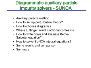
Auxiliary particle method How to set up perturbation theory? How to choose diagrams? Where Luttinger Ward functional comes in? How to write down end evaluate Bethe-Salpeter equation? How to solve SUNCA integral equations? Some results and comparison Summary Diagrammatic auxiliary particle impurity solvers - SUNCA
Advantages/Disadvantages • Advantages: • Fast (compared to QMC) IS with no additional time cost for large N • Defined and numerically solved on real axis (more information) • Disadvantages: • Not exact and needs to be carefully tested and benchmarked • (breaks down at low temperature T<<Tk – but gets • better with increasing N) • No straightforward extension to a non-degenerate AIM (relays on • degeneracy of local states) – but straightforward extension to • out-of-equilibrium AIM
Problems solving SUNCA • Usual perturbation theory not applicable (no conservation of fermions) • slightly modified perturbation carefully determine sign and prefactor • Two projections: • exact projection on the pysical hilbert space • need to project out local states with energies far from • the chemical potential • Numerics! • Solve Bethe-Salpeter equation with singular kernel • Pseudo particles with threshold divergence – • need of non-equidistant meshes • Integration over T-matrices that are defined on non-equidistant mesh
Exact diagonalization of the interacting region (impurity site or cluster) Introduction of auxiliary particles # electrons in even is boson # electrons in odd is fermion Local constraint (completeness relation) for pseudo particles: Diagrammatic auxiliary particle impurity solvers
Local constraint and Hamiltonian Representation of local operators Hamiltonian in auxiliary representation local hamiltonian quadratic (solved exactly) bath hamiltonian is quadratic perturbation theory in coupling between both possible
Remarks • Why do we introduce “unnecessary” new degrees of freedom? • (auxiliary particles) • Interaction is transferred from term U to term V Coulomb repulsion U is usually large and V is small But the perturbation in V is singular! • Unlike the Hubbard operator, the auxiliary particles are fermions and bosons and the Wick’s theorem is valid Perturbation expansion is possible
Diagrammatic solutions • Since the perturbation expansion in V is singular it is desirable to • sum infinite infinite number of diagrams (certain subclass). This is • necessary to get correct low energy manybody scale TK . • Definition of the approximation is done by defining the Luttinger-Ward • functional : Fully dressed pseudoparticle Green’s functions • Procedure guarantees that the approximation is conserving • for example:
Infinite U AIM within NCA • Gives correct energy scale • Works for T>0.2 TK • Below this temperature Abrikosov-Suhl resonance exceeds unitarity limit • Gives exact non-Fermi liquid exponents in the case of 2CKM • Naive extension to finite U very badly fails • TK several orders of magnitude too small
How to extend to finite U? Schrieffer-Wolff transformation
To get correct energy scale for infinite U AIM, self-consistent method is needed Infinite series of skeleton diagrams is needed to recover correct low energy scale of the AIM at finite Coulomb interaction U The method can be extended to multiband case (with no additional effort) Diagrammatic method can be used to solve the cluster DMFT equations. Summary
Exact projection onto Q=1 subspace • Hamiltonian commutes with Q Q constant in time • Q takes only integer values (Q=0,1,2,3,...) • How to project out only Q=1? • Add Lagrange multiplier If then Proof:
Exact projection in practice How can we impose limit analytically? Only integral around branch-cut of bath Green’s function survives (bath=Green’s functions of quantities with nonzero expectation value in Q=0 subspace) Exact projection is done analytically!
Physical quantities Exact relation: Dyson equation: In grand-canonical ensemble