
Optimisation
E N D
Presentation Transcript
Optimisation Derivative-free optimization: From Nelder-Mead to global methods
Definition • Optimizing a function is looking for the set of values of the variables that will maximize (or minimize) the function. • Optimization is usually a very complex problem. There are many different techniques, each being adapted to a specific kind of problems. • There is no universal method, but a set of tools which requires a lot of experience to be used properly.
Optimization caracteristics • Global/local optimization • Global optimization is searching for the absolute extremum of the function over its entire definition domain • Local optimization is looking for the extremum of the function in the vicinity of a given point • Stochastic / deterministic methods • A stochastic method searches the definition domain of the function in a random way . Two succesive runs can give different résults. • A deterministic method always walks the search space in the same way, and always gives the same results.
Derivation (deterministic) • When it is possible to compute and solve f’(x)=0, then we know that the extrema of the function are in the set of solutions. • This method can only be used for very simple analytic functions
Gradient method (deterministic and local) If f(X) is a real valued function of a real valued vector X, and we can calculate f’(X), we compute: Xn+1 = Xn - a f’(Xn), a>0 The best choice of a>0 is done by minimizing: G(a)=f(Xn– a f’(Xn)) It’s usually impossible to solve the above equation and approximate methods are used.
Local, deterministic, order 2, methods. • To accelerate computation we use the computation of the first and second order derivatives of the function • We need to be able to compute both, in a reasonnable amount of time.
Local, deterministic, order 2, methods. • f(y) = f(x) + f’(x) (y-x) + ½ f’’(x) (y-x)2 + d • We minimize the y quadratic form: • f’(x)+f’’(x)(y-x)=0 => y = x – f’(x)/f’’(x) • Algorithm: • xn+1 = xn – f’(xn) / f’’(xn) • Known as Newton method • Convergence is (much) faster than the simple gradient method.
Deterministic method: BFGS • BFGS approximates the hessian matrix without explicitly computing the hessian • It only requires knowledge of the first order derivative. • It’s faster than gradient, slower (but much more practical) than Newton • One of the most used method.
Local deterministic: Nelder-Mead simplex • Works by building an n+1 points polytope for an n variables function, and by shrinking, expanding and moving the polytope. • There’s no need to compute the first or second order derivative, or even to know the analytic form of f(x), which makes NMS very easy to use. • The algorithm is very simple.
Nelder-Mead simplex • Choose n+1 points (x1,..xn+1) • Sort: f(x1)<f(x2)…<f(xn+1) • Compute barycenter: x0 = (x1+…+xn)/n • Reflection of xn+1/x0: xr=x0+(x0-xn+1) • If f(xr)<f(x1), xe=x0+2(x0-xn+1). If f(xe)<f(xr), xn+1<-xe, else xn+1<-xr, back to sort. • If f(xn)<f(xr), xc=xn+1+(x0-xn+1)/2.If f(xc)<f(xr) xn+1<-xc, back to sort • Otherwise: xi <- x0+(xi-x1)/2. Back to sort.
Stochastic optimization • Do not require any regularity (functions do no even need to be continuous) • Usually expensive regarding computation time, and do not guarantee optimality • There are some theoretical convergence results, but they usually don’t apply in day to day problems.
Simulated annealing • Generate one random starting point x0inside the search space. • Build xn+1=xn+B(0,s) • Compute: tn+1=H(tn) • If f(xn+1)<f(xn) then keep xn+1 • If f(xn+1)>f(xn) then : • If |f(xn+1)-f(xn)|<e- k t then keep xn+1 • Si |f(xn+1)-f(xn)|>e- k t then keep xn
Important parameters • H (the annealing schedule): • Too fast=>the algorithm converges very quickly to a local minimum • Too slow=>the algorithm converges painfully slowly. • Deplacement: B(0,s) must search the whole space, and mustn’t jump too far or too close either
Efficiency • SA can be useful on problems too difficult for « classical methods » • Genetic algorithms are usually more efficient when it is possible to build a « meaningful » crossover
Genetic algorithms (GA) • Search heuristic that « mimics » the process of natural evolution: • Reproduction/selection • Crossover • Mutation • John Holland (1960/1970) • David Goldberg (1980/1990).
Coding / population generation • If x is a variable of f(x), to optimize on the interval [xmin,xmax]. • We rewrite x :2n (x-xmin)/(xmax-xmin) • This gives an n bits string: • For n=8: 01001110 • For n=16: 0100010111010010 • A complete population of N (n bits string) is generated.
Crossover • Two parents : • 01100111 • 10010111 • One crossover point (3): • 011|00111 • 100|10111 • Two children: • 011|10111 • 100|00111
Mutation • One randomly chosen element: • 01101110 • One mutation site (5): • 01101110 • Flip bit value: • 01100110
Reproduction/selection • For each xi compute f(xi) • Compute S=S(f(xi)) • Then for each xi : • p(xi)=f(xi)/S • The n elements of the new population are picked from the pool of the n elements of the old population with a bias equal to p(xi). • Better adapted elements are more reproduced
Exemple de reproduction • f(x)=4x(1-x) • x in [0,1[
AG main steps • Step 1: reproduction/selection • Step 2: crossing • Step 3: mutation • Step 4: End test.
Scaling • Fact: in the « simple » AG, the fitness of an element x is equal to f(x) • Instead of using f(x) as fitness, f is « scaled » by using an increasing function. • Exemples: • 5 (f(x)-10)/3: increase selection pressure • 0.2 f + 20 : diminishes selection pressure • There are also non-linear scaling functions
Sharing • Selection pressure can induce too fast convergence to local extrema. • Sharing modifies fitness depending on the number of neighbours of an element: • fs(xi)=f(xi)/Sj s(d(xi,xj)) • s is a decreasing function. • d(xi,xj) is a distance measurement between i et j
Sharing • To use sharing, you need a distance function over variables space • General shape of s:
Bit string coding problem • Two very different bit strings can represent elements which are very close to each other: • If encoding real values in [0,1] with 8 bits: • 10000000 et 01111111 represent almost the same value (1/2) but their hamming distance is maximal (8). • Necessity to use Grey encoding.
Using a proper coding • For real variable functions, real variable encoding is used • Crossover: • y1 = a x1 + (1-a) x2 • y2 = (1-a) x1 + a x2 • a randomly picked in [0.5,1.5] • Mutation: • y1 = x1 + B(0,s)
Modeling • Only one manoeuver maximum by aircraft • 10, 20 or 30 degrees deviation right or left • Then return to destination • Offset • Variables: 3 n • T0: start of manoeuver • T1: end of manoeuver • A: angle of deviation • Uncertainties on speeds