1 / 0

Welcome to the R intro Workshop

Welcome to the R intro Workshop. Before we begin, please download the “SwissNotes.csv” and “cardiac.txt” files from the ISCC website, under the Introduction to R workshop to the desktop of your computer. www.iub.edu/~iscc/workshops.html.

misha
Download Presentation

Welcome to the R intro Workshop

An Image/Link below is provided (as is) to download presentation Download Policy: Content on the Website is provided to you AS IS for your information and personal use and may not be sold / licensed / shared on other websites without getting consent from its author. Content is provided to you AS IS for your information and personal use only. Download presentation by click this link. While downloading, if for some reason you are not able to download a presentation, the publisher may have deleted the file from their server. During download, if you can't get a presentation, the file might be deleted by the publisher.

E N D

Presentation Transcript


  1. Welcome to the R intro Workshop Before we begin, please download the “SwissNotes.csv” and “cardiac.txt” files from the ISCC website, under the Introduction to R workshop to the desktop of your computer. www.iub.edu/~iscc/workshops.html
  2. Introduction to RWorkshop in Methods from the Indiana Statistical Consulting Center

    Thomas A. Jackson October 11, 2013
  3. Overview The R Project for Statistical Computing http://cran.r-project.org “R is a language and environment for statistical computing and graphics. It is a GNU project which is similar to the S language and environment which was developed at Bell Laboratories (formerly AT&T, now Lucent Technologies) by John Chambers and Colleagues. R can be considered as a different implementation of S. There are some important differences, but much code written for S runs unaltered under R.” - Description from CRAN Website
  4. Benefits R … is free is interactive: we can type something in and work with it How we analyze data can be broken into small steps is interpretative: we give it commands and it translates them into mathematical procedures or data management steps can be used in a batch: nice because it is documented is a calculator: it is unlike other calculators though because you can create variables and objects
  5. Let’s Get R Started How to open R → Start Menu → Programs → Departmentally Supported → Stat/Math → R
  6. Graphical User Interface (GUI) Three Environments Command Window (aka Console) Script Window Plot Window
  7. Command Window Basics To quit: type q() Save workspace image? Moves from memory to hard-drive Storing variable in memory <- , -> , or = a<- 5 stores the number 5 in the object “a” pi -> b stores the number π= 3.141593 in “b” x = 1 + 2 stores the result of the calculation (3) in “x” “=“ requires left-hand assignment Try not to overwrite reserved names such as t, c, and pi!
  8. Command Window Basics Printing to output Calculations that are not stored print to output > 3 + 5 [1] 8 Type name to view stored object > a [1] 5 Use print() > print(a) [1] 5 View objects in workspace objects() or ls()
  9. Command Window Basics Clearing the console (command window) Mac: Edit → Clear Console Windows: Edit → Clear Console or Mac: Alt + Command + L Windows: Ctrl + L Removing variables from memory rm() or remove() > x <- 4 > rm(x) rm(list = ls()) remove all variables
  10. Script Window Basics Saving syntax (code) Mac: File → New Windows: File → New Script Documenting code: # Comments out everything on line behind Running code from Script Window Mac: Apple + Enter Windows: F5 or Ctrl + r
  11. Working Directory Obtaining working directory getwd() Mac: Misc → Get Working Directory Windows: File → Change dir... Changing working directory setwd() Mac: Misc → Change Working Directory Windows: File → Change dir...
  12. Path Names Specify with forward slashes or double backslashes Enclose in single or double quotation marks Examples setwd(“C:/Users/jacksota/Desktop”) setwd(‘C:\\Users\\jacksota\\Desktop’)
  13. Try it! #1 From the command window find your current working directory. Change the working directory to be the Desktop folder under your Username. Save the commands for finding and changing the working directory to the desktop in a script file. Save the script to the desktop.
  14. R Help Helpful commands If you know the function name: help() or ? > help(log) > ?exp If you do not know the function name: help.search() or ?? > help.search(“anova”) > ??regression
  15. Documentation Elements of a documentation file Function{Package} Description Usage: What your code should look like, “=“ gives default Arguments: Inputs to the function Details Value: What the function will return See Also: Related functions Examples
  16. Online Resources CRAN Website: http://cran.r-project.org/ R Seek: http://www.rseek.org/ Quick-R tutorial: http://www.statmethods.net/ R Tutor: http://www.r-tutor.com/ UCLA: http://www.ats.ucla.edu/stat/r/ R listservs Google Google tip: include “[R]” (instead of just “R”) with search topic to help filter out non-R websites
  17. Additional Packages Over 4,900 listed on the CRAN website! Use with caution Initial download of R: base, graphics, stats, utils 1) Installing a package: Mac: Packages & Data → Package Installer Use Package Search to locate and press ‘Install Selected’ Windows: Packages → Install Packages Locate desired package and press ‘OK’ install.packages(“MASS”) 2) Using an installed package: You MUST call it into active memory with library() > library(MASS)
  18. Try it! #2 1) Using help() or ?, open the documentation for plot table eigen 2) Locate and install the psych package
  19. Data Structures R has several basic types (or “classes”) of data: Numeric - Numbers Character – Strings (letters, words, etc.) Logical – TRUE or FALSE Vector Matrix Array Data Frame List NOTE: There are other classes, but these are most common. Understanding differences will save you some headache.
  20. Data Structures Find class of data Unknown class: class() Check particular class: is.“classname”() > a <- 5 > class(a) [1] “numeric” > is.character(a) [1] FALSE Change class: as.classname() > as.character(a) [1] “5”
  21. Vectors Combine items into vector: c() > c(1,2,3,4,5,6) [1] 1 2 3 4 5 6 Repeat number of sequence of numbers: rep() > rep(1,5) [1] 1 1 1 1 1 > rep (c(2,5,7), times = 3) [1] 2 5 7 2 5 7 2 5 7
  22. Vectors Sequence generation: seq() > seq(1,5) [1] 1 2 3 4 5 > seq(1,5, by = .5) [1] 1.0 1.5 2.0 2.5 3.0 3.5 4.0 4.5 5.0 Try 1:10 or 10:1
  23. Matrices Create matrix: matrix() 6 x 1 matrix: matrix(1:6, ncol = 1) 2 x 3 matrix: matrix(1:6, nrow =2, ncol =3) 2 x 3 matrix filling across rows first: matrix(1:6, nrow = 2, ncol = 3, byrow = TRUE) Create matrix of more than two dimensions (array): array()
  24. Lists Create a list: list() Holds vectors, matrices, arrays, etc. of varying lengths Objects in the list can be named or unnamed > list(matrix(0, 2, 2), y = rep(c(“A”, “B”), each = 2)) [[1]] [,1] [,2] [1,] 0 0 [2,] 0 0 $y [1] “A” “A” “B” “B” Data Frame: specialized list that holds variables of same length
  25. Data Frames Create a data frame: data.frame() Like a matrix, holds specified number of rows and columns > x <- 1:4 > y <- rep(c(“A”, ”B”), each = 2) > data.frame(x,y) x y 1 1 A 2 2 A 3 3 B 4 4 B Unnamed variables get assigned names > data.frame(1:2, c(“A”, “B”)) X1.2 c..A….B.. 1 1 A 2 2 B
  26. Try It! #3 Enter the following data into R: CHI 11.65 23.84 FRA 10.73 21.99 GER 10.81 21.71 1) Try to enter the data above as a data frame 2) Can you enter it as a matrix? Would the data be different in a matrix, rather than a dataframe?
  27. Basic Operations Arithmetic: +, -, *, / Order of operations: () Exponentiaition: ^, exp() Other: log(), sqrt Evaluate standard Normal density curve, at x = 3 > x <- 3 > 1/sqrt(2*pi)*exp(-(x^2)/2) [1] 0.004431848
  28. Vectorization R is great at vectorizing operations Feed a matrix or vector into an expression Receive an object of similar dimension as output For example, evaluate at x = 0,1,2,3 > x <- c(0,1,2,3) > 1/sqrt(2*pi)*exp(-(x^2)/2) [1] 0.39842280 0.241970725 0.053990967 0.004431848
  29. Logical Operations Compare: ==, >, <, >=, <=, != > a <- c(1,1,2,4,3,1) > a == 2 [1] FALSE FALSE TRUE FALSE FALSEFALSE And: & or && Or: | or || Find location of TRUEs: which() > which(a == 1) [1] 1 2 6
  30. Subsetting > a <- 1:5 > b <- matrix(1:12,nrow = 3) Use Square brackets [] Pick range of elements: a[1:3] Pick particular elements: a[c(1,3,5)] Do not include elements: a[-c(1,4)]
  31. Subsetting (cont.) Use commas in more than on dimension (matrices & data frames) Pick particular elements: B[1:2,2:4] Give all rows and specified columns: B[,1:2] Give all columns and specified rows: B[1:2,] Note: B[2] coerces into a vector then gives specified element
  32. Reading External Data Files SwissNotes.csv Data set Complied by Bernard Flury Contains measurements on 200 Swiss Bank Notes 100 genuine and 100 counterfeit notes
  33. Reading External Data Files (cont.) Most general function: read.table() read.table(file,header=FALSE,sep = “”,…) Creates a data frame File name must be in quotes, single or double File name is case sensitive Include file name extension if data not in working directory > read.table(“C:\\Users\\jacksota\\Desktop\\SwissNotes.csv”,T,“,”) > read.table(“SwissNotes.csv”,T,“,”), if we have set the working dir. correctly Don’t know the file extension? Try: file.choose() > read.table(file.choose(), header = TRUE, sep = ”,”) sep defines the separator, e.g. “,” or “\t” or “” header indicates variable names should be read from first row
  34. Reading External Data Files For comma delimited files: read.csv() For tab delimited files: read.delim() For Minitab, SPSS, SAS, STATA, etc. data: foreign package Contains functions to read variety of file formats Functions operate like read.data() Contains functions for writing data into these file formats
  35. Data Frame Hints Identify variable names in data frame: names() > data1 <- read.table(“SwissNotes.csv”, sep=“,”, header =TRUE) > names(data1) [1] “Length” “LeftHeight” “RightHeight” “LowerInner.Frame” [5] “UpperInner.Frame” “Diagonal” “Type” Assign name to data frame variables > names(data1) <- c(“Length”, “LeftHeight”, “RightHeight”, “LowerInner..Frame”, “UpperInner.Frame”, “Diagonal”, “Type”) Note: names are strings and MUST be contained in quotes
  36. Data Frame Hints (cont.) Create objects out of each data frame variable: attach() In the Swiss Note data, to refer to Type as its own object > attach(data1) > Type [1] Genuine GenuineGenuine ….
  37. Data Frame Hints (cont.) Remove attached objects from workspace: detach() > detach(data1) > Type Error: object “Type” not found Note: Type is still part of original data frame, but is no longer a separate object.
  38. Try It! #4 Caridac.txt includes measurements taken to predict cardiac events, such as heart attacks. You should have already downloaded it and saved to your desktop Tab delimited data set (sep=“\t”) with header Read cardiac.txt into R Select data for male participants only For male participants, select data for basal heart rate (bhr) and peak heart rate (pkhr) only
  39. plot() function plot() is the primary plotting function Calling plot will open a new plotting window Documentation: ?plot For complete list of graphical parameters to manipulate: ?par
  40. plot() function Let’s visualize the SwissNotes.csv data. After loading the data into R, attach the data frame using attach(data). Let’s try a scatter plot of LeftHeight by RightHeight. >plot(LeftHeight, RightHeight)
  41. plot() function Change symbols: Option pch=. See ?par for details. >plot(LeftHeight,RightHeight,pch=2)
  42. plot() Function Change symbol color: Option col= Specify by number or by name: col=2 or col=“red” Hint: Type palette() to see colors associated with number Type colors() to see all possible colors > plot(LeftHeight, RightHeight, col=“red”)
  43. What types of points can we get?
  44. plot() Function Change plot type: Option type = “p” for points “l” for lines “b” for both “c” for lines part alone of “b” “o” for both overplotted “h” for histogram like (or high-density) vertical lines “s” for stair steps “S” for other steps, see Details below “n” for no plotting
  45. Plot() Function Points with lines…works better on sorted list of points >plot(LeftHeight,RightHeight,type=“o”)
  46. Scatterplots for Multiple Groups Use plot() with points() to plot different groups in same plot Genuine notes vs. Counterfeit notes >plot(LeftHeight[Type==“Genuine”],Rightheight[Type==“Genuine”], col=“red”) >points(LeftHeight[Type==“Counterfeit”],RightHeight[Type==“Counterfeit”] ,col=“blue”)
  47. Axis Labels and Plot Titles The plot() command call has options to Specify x-axis label: xlab = “X Label” Specify y-axis label: ylab = “Y Label” Specify plot title: main = “Main Title” Specify subtitle: sub = “Subtitle”
  48. Axis Labels and Plot Titles >plot(LeftHeight[Type==”Genuine”],RightHeight[Type==“Genuine”], col=“red”,main=“Plot of Bank Note Heights”,sub=“Measurements are in mm”,xlab=“Height of Left Side”,ylab=“Height of Right Side”) >points(LeftHeight[Type==“Counterfeit”], RightHeight[Type=“Counterfeit”],col=“blue”)
  49. Legends legend(“topleft”,c(“Genuine Notes”, ”Counterfeit Notes”),pch=c(21,21),col=c(“red”,”blue”))
  50. Try It! Using the cardiac data set, try the following exercises Create a scatterplot of age vs. peak heart rate (pkhr). Be sure to label your axes and title the plot. Using information available on the points() documentation page, adjust your scatterplot to have symbols that are filled blue squares. In your age versus peak heart rate scatterplot, plot the males and females with different symbols and different colors. Add a legend to your plot.
  51. Adding Lines To add straight lines to plot: abline() abline() refers to standard equation for a line: y = bx + a Horizontal line: abline(h= ) Vertical Line: abline(v= ) Otherwise: abline(a= , b= ) or abline(coef=c(a,b))
  52. Adding Lines > abline(coef=c(21.7104,0.8319))
  53. Histograms Histograms are another popular plotting option. > hist(Length)
  54. pairs() Function Using the SwissNote Data > pairs(swiss)
  55. Boxplots To create boxplots: boxplot() Specify one or more variables to plot. > boxplot(swiss$Length) > boxplot(swiss[,2:3])
  56. Boxplots Use a formula specification for side-by-side boxplots. Note: boxplot() has many options, e.g. notches. See ?boxplot. > boxplot(Length~Type,notch=TRUE,data=swiss)
  57. Try It! Using the cardiac data set, try the following exercises Create histograms for basal blood pressure (basebp) and systolic blood pressure (sbp). Try creating boxplots of the same variables. Can you do separate plots for Males and Females?
  58. Mean or Average Mean() > mean(swiss[,”Length”]) > mean(swiss) rowMeans() > rowMeans(swiss[,1:6]) colMeans > colMeans(swiss[,7])
  59. Variability Variance: var() > var(swiss[,”Length”]) > var(swiss) Covariance() > cov(swiss) Correlation() > cor(swiss[,1:6]) Standard deviation > sd(swiss$length)
  60. Five-number Summary >summary(swiss[1:3]) Length LeftHeightRightHeight Min. :213.8 Min. :129.0 Min. :129.0 1st Qu.:214.6 1st Qu.:129.9 1st Qu.:129.7 Median :214.9 Median :130.2 Median :130.0 Mean :214.9 Mean :130.1 Mean :130.0 3rd Qu.:215.1 3rd Qu.:130.4 3rd Qu.:130.2 Max. :216.3 Max. :131.0 Max. :131.1
  61. Creating Tables table() produces crosstabs of factors or categorical variables Using the cardiac data: > table(cardiac[,7:9]) , , newMI = 0 chestpain gender 0 1 F 6 10 M 4 8 , , newMI = 1 chestpain gender 0 1 F 100 222 M 62 146
  62. Try It! Using the cardiac data Find the descriptive statistics for the chestpain (chestpain) and dose (dose). Note that chestpain is categorical (0=no chest pain, 1=chest pain) and that does is continuous.
  63. Univariate t-tests t.test() produces 1- and 2-sample (paired or independent) t-tests. 1-sample t-test > t.test(x,alternative=“two.sided”,mu=0,conf.level=0.95) 2 independent samples t-test > t.test(x,y,alternative=“two.sided”,mu=0,paired=FALSE, conf.level=0.95) paired t-test > t.test(x,y,alternative=“two.sided”,mu=0,paired=TRUE, var.equal=TRUE,conf.level=0.95)
  64. 2 Independent Samples t-test x: diagonal measurements for Genuine bank notes y: diagonal measurements for Counterfeit bank notes > x = swiss[Type==“Genuine”,”Diagonal”] > y = swiss[Type==“Counterfeit”,”Diagonal”] > t.test(x,y,alternative=“greater”,mu=0, paired=FALSE,var.equal=TRUE)
  65. 2 Independent Samples t-test > t.test(x,y,alternative=“greater”,mu=0, paired=FALSE,var.equal=TRUE) Two Sample t-test data: x and y T = 28.9149, df = 198, p-value < 2.2e-16 alternative hypothesis: true difference in means is greater than 0 95 percent confidence interval: 1.948864 Inf sample estimates: mean of x mean of y 141.517 139.450
  66. Try It! #8 Using the cardiac data Using the appropriate t-tests, test the following hypotheses H0: μage = 72 vs. H1: μage < 72 For peak heart rate (pkhr), H0: μmale = μfemale vs. H1: μmale > μfemale For peak heart rate, H0: μno chest pain = μchest pain vs. H1: μno chest pain ≠ μchest pain
  67. Generating Random Numbers R contains functions for generating random numbers from many well-known distributions. Random number from standard normal distribution: > rnorm(1,mean=0,sd=1) [1] 0.5308293 Vector of random numbers from uniform distribution: > runif(3, min=0, max=1) [1] 0.6578880 0.3261863 0.3093383 To reproduce results: set.seed()
  68. Function Basics if() statement > n = rnorm(1) > if(n < 0){ n = abs(n) } if() statement with else() > n = rnorm(1) >if (n < 0){ n = abs(n) } else{n = 0}
  69. Function Basics for() loop > temp = rep(0,10) > for (i in 1:10){ temp[i] = i+1 } > temp [1] 2 3 4 5 6 7 8 9 10 11
  70. Function Basics while() loop > n = 1 > while (n < 10 ){ n = n+1 }
  71. Creating Functions test.function = function(input arguments){ commands to execute }
  72. Creating Functions For example, let’s define a new function average to find the average of a set of numbers. average = function(x){ n = length(x) average = sum(x)/n print(average) }
  73. Sourcing After writing a function in a script file, bring it into working memory using source(). Source(“pathname/test.function.R”)
More Related