Download
1 / 30
320 likes | 559 Views
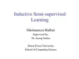
DTW-D : Time Series Semi-Supervised Learning from a Single Example. Yanping Chen. Outline. Introduction The proposed method The key idea When the idea works Experiment. Introduction. Most research assumes there are large amounts of labeled training data .

E N D
DTW-D: Time Series Semi-Supervised Learning from a Single Example Yanping Chen
Outline • Introduction • The proposed method • The key idea • When the idea works • Experiment
Introduction • Most research assumes there are large amounts of labeled training data. • In reality, labeled data is often very difficult /costly to obtain • Whereas, the acquisition of unlabeled data is trivial Example: Sleep study test A study produce 40,000 heartbeats; but it requires cardiologists to label the individual heartbeats;
Introduction • Obvious solution: Semi-supervised Learning (SSL) • However, direct applications of off-the-shelf SSL algorithms do not typically work well for time series
Our Contribution • explain why semi-supervised learning algorithms typically fail for time series problems • 2. introduce a simple but very effective fix
Outline • Introduction • The proposed method • The key idea • When the idea works • Experiment
SSL: self-training Self-training algorithm: 1. Train the classifier based on labeled data 2. Use the classifier to classify the unlabeled data 3. the most confident unlabeled points, are added to the training set. 4. The classifier is re-trained, and repeat until stop criteria is met classifier classify retrain train P:Labeled U:unlabeled Evaluation: The classifier is evaluated on some holdout dataset
Two conclusions from the community • Most suitable classifier: the nearest neighbor classifier(NN) • Distance measure: DTW is exceptionally difficult to beat • In time series SSL, we use NN classifier and DTW distance. • For simplicity, we consider one-class classification, positive class and negative class. [1] HuiDing, GoceTrajcevski, Peter Scheuermann, Xiaoyue Wang and Eamonn Keogh (2008) Querying and Mining of Time Series Data: Experimental Comparison of Representations and Distance Measures, VLDB 2008
Our Observation labeled unlabeled • Observation: • Under certain assumptions, unlabeled negative objects are closer to labeled dataset than the unlabeled positive objects. • Nevertheless, unlabeled positive objects tend to benefit more from using DTW than unlabeled negative objects. • The amount of benefit from DTW over ED is a feature to be exploited. • I will explain this in the next four slides dpos dneg dneg < dpos
Our Observation 1 1 P: Labeled Dataset Example: Positive class 0 0 P1 Negative class U: unlabeled dataset U1 U2
Our Observation 1 1 P: Labeled Dataset U: Unlabeled Dataset 0 0 U1 P1 U U2 Ask any SSL algorithm to choose one object from U to add to P using the Euclidean distance. Not surprising, as is well-known,ED is brittle to warping[1]. U2 U1 P1 P1 ED(P1, U1) = 6.2 ED(P1,U2) = 11 ED(P1, U1) < ED(P1,U2) , SSL would pick the wrong one. [1[ Keogh, E. (2002). Exact indexing of dynamic time warping. In 28th International Conference on Very Large Data Bases. Hong Kong. pp 406-417.
Our Observation 1 1 0 0 U1 P1 P U U2 Why DTW fails? Besides warping, there are other differencebetweenP1and U2 . E.g., the first and last peak have different heights. DTW can not mitigate this. What about replacing EDwithDTWdistance? U2 U1 P1 P1 DTW(P1, U1) = 5.8 DTW(P1,U2) = 6.1 DTW helps significantly, but still picks the wrong one.
Our Observation 1 1 P1 P 0 0 U1 U U2 ED: U2 U1 ED(P1, U1) = 6.2 ED(P1,U2) = 11 P1 P1 DTW: U2 Under the DTW-Delta ratio(r): U1 P1 P1 DTW(P1, U1) = 5.8 DTW(P1,U2) = 6.1
Why DTW-D works? Objects from different classes: Objects from same class: shape difference warping noise distance from: + ED = shape difference + + warping noise warping noise ED = shape difference noise DTW = + noise DTW = warping noise For objects from same class: DTW-D = For objects from different classes: DTW-D= Thus, intra-class distance is smaller than inter-class distance, and a correct nearest neighbor will be found.
DTW-D distance • DTW-D: the amount of benefit from using DTW over ED. - • Property:
Outline • Introduction • The proposed method • The key idea • When the idea works • Experiment
When does DTW-D help? Two assumptions Platonic ideal • Assumption 1: The positive class contains warped versions ofsome platonic ideal, possibly with other types of noise/distortions. Warped version • Assumption 2: The negative class is diverse, and occasionally produces objects close to a member of the positive class, even under DTW. • Our claim: if the two assumptions are true for a given problem, DTW-D will be better than either ED or DTW.
When are our assumptions true? • Observation1: Assumption 1 is mitigated by large amounts of labeled data U: 1 positive object, 200 negative objects(random walks). P: Vary the number of objects in P from 1-10, and compute the probability that the selected unlabeled object is a true positive. Result: When |P| is small, DTW-D is much better than DTW and ED. This advantage is getting less as |P| gets larger.
When are our assumptions true? • Observation2: Assumption 2 is compounded by a large negative dataset Positive class Negative class P: 1 positive object U: We vary the size of the negative dataset from 100 -1000. 1 positive object. Result: When the negative dataset is large, DTW-D is much better than DTW and ED.
When are our assumptions true? • Observation3: Assumption 2 is compounded by low complexity negative data 5 non-zero DFT coefficients; 20 non-zero DFT coefficients; P: 1 positive object U: We vary the complexity of negative data, and 1 positive object. Result: When the negative data are of low complexity, DTW-D is better than DTW and ED. [1] Gustavo Batista, Xiaoyue Wang and Eamonn J. Keogh (2011) A Complexity-Invariant Distance Measure for Time Series. SDM 2011
Summary of assumptions • Check the given problem for: • Positive class • Warping • Small amounts of labeled data • Negative class • Large dataset, and/or… • Contains low complexity data
DTW-D and Classification • DTW-D helps SSL, because: • small amounts of labeled data • negative class is typically diverse and contains low-complexity data • DTW-D is not expected to help the classic classification problem: • large set of labeled training data • no class much higher diversity and/or with much lower complexity data than • other class
Outline • Introduction • The proposed method • The key idea • When the idea works • Experiment
Experiments • Initial P: • Single training example • Multiple runs, each time with a different training example • Report average accuracy • Evaluation • Classifier is evaluated for each size of |P| select U P test holdout
Experiments • Insect Wingbeat Sound Detection Two positive examples Unstructured audio stream Two negative examples Positive :Culexquinquefasciatus♀ (1,000) Negative : unstructured audio stream (4,000) DTW-D 1 0.8 DTW 0.6 • Accuracy of classifier 0.4 0.2 ED 0 200 1000 2000 0 100 200 300 400 Number of labeled objects in P
Comparison to rival methods Both rivals start with 51labeled examples Our DTW-D starts with a singlelabeled example 1 0.95 0.9 Ratana’s method[1] • Accuracy of classifier 0.85 Wei’s method[2] 0.8 Grey curve: The algorithm stops adding objects to the labeled set 0.75 0.7 0 50 100 150 200 250 300 350 400 • Number of objects added to P • [1]W. Li, E. Keogh, Semi-supervised time series classification, ACM SIGKDD: 2006 • [2] C. A. Ratanamahatana., D.Wanichsan, Stopping Criterion Selection for Efficient Semi-supervised Time Series Classification. SNPD 2012. 149: 1-14, 2008.
Experiments • Historical Manuscript Mining Positiveclass: Fugger shield(64) Negative class: Other image patches(1,200) 1 DTW-D 0.9 DTW 0.8 • Accuracy of classifier 0.7 ED Red Green Blue 0.6 0.5 0 2 4 6 8 10 12 14 16 Number of labeled objects in P
Experiments • Activity Recognition 0.6 DTW-D 0.5 DTW 0.4 • Accuracy of classifier 0.3 ED 0.2 0.1 0 10 20 30 40 50 60 70 80 90 100 Number of labeled objects in P Dataset: Pamap dataset[1] (9 subjects performing 18 activities) Positive class: vacuum cleaning Negative class: Other activities • [1] PAMAP, Physical Activity Monitoring for Aging People, www.pamap.org/demo.html , retrieved 2012-05-12.
Conclusions • We have introduced a simple idea that dramatically improves the quality of SSL in time series domains • Advantages: • Parameter free • Allow use of existing SSL algorithm. Only a single line of code needs to be changed. • Future work: • revisiting the stopping criteria issue • consider other avenues where DTW-D may be useful
Questions? Thank you! Contact Author: Yanping Chen Email: ychen053@ucr.edu