Download
1 / 35
360 likes | 709 Views
Inputs: Factors of Production. Factors of production: Land Labor Capital Intermediate goods (Entrepreneurial Services ) Production Costs = Costs of Inputs . Production in the Short Run versus Production in the Long Run .

E N D
Inputs: Factors of Production Factors of production: • Land Labor Capital • Intermediate goods • (Entrepreneurial Services ) • Production Costs = Costs of Inputs
Production in the Short Runversus Production in the Long Run • In the short run at least one of the factors of production remains unchanged (fixed). • In the long run all factors of production are variable. • In a two-input production process, in the short run, only oneinput is variable. • In a two-input production model, in the short run, the changes in the output (physical product) are the result of changes in the variable input.
Production in the Long Run • In the long run all inputs used in the production process by the firm are variable. • In a two-input production model, in the long run, both inputs (say, capital and labor) are variable. • In the long run the level of the output of a firm can change as a result of changes in any or all inputs.
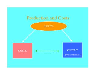
A Short-Run Production (Function) Analysis Our model: A firm using two inputs: Capital (K); Fixed Input Labor (L); Variable input We examine the relationship between the variable input (labor) and the output. We examine how changes in labor (the variable input) affect the out put.
Output Measures • Total (Physical) Product (output), TPP: The total amount of output produced by the firm over a certain period • Average (Physical) Product (of the variable input), APP: Total (Physical) Product divided by the number units of the variable input • Marginal (Physical) Product (of the variable input), MPP: The change in total product resulting from employing one additional unit of the variable input
Production in the Short Run P. P. P.
MPP and APP Change in TPP Marginal Physical Product = MPP = Change in V. Input Total Physical Product Average Physical Product = APP = Total V. Input
The “Law” of Diminishing Return • Increases in the amount of any one input, holding the amounts all other inputs constant, would eventually result in decreasing marginal product of the variable input. Explanation: Unless all inputs are perfectly and infinitely substitutable, as we increase the amount of one input, while keeping other inputs constant, at some point the productive effectiveness of that input starts to decline.
Choosing the Optimal Mix of Inputs • One approach to choosing the optimal (least costly) mix of inputs is to compare the (marginal) cost of producing one extra unit of out put across different inputs. • The firm would likely use the input that increases its output at the lowest cost by comparing Input Price across all available inputs. MPP
Isoquant and Isocost Q = f ( K, L) Cost = rK + w L where r = price of capital w = wage
Isoquant K Slope = MPL/MPK = MRTS Q4 Q3 Q2 L Q1 0
Isocost K Cost = r.K +w. L Cost/r Slope = w/r L 0 Cost/w
Isocost K Cost = r.K +w. L Cost/r Slope = w/r Q2 Q1 L 0 Cost/w
Input Optimizing Rule MPL MPK MPM --------- = --------- = --------- w r PM or, MPL w MPL w ------ = -------- , ---------- = --------- MPM r MPM PM
X path K Cost/r Q2 Q1 L 0 Cost/w
$TC LTC Q o
$ LTC LAC = LTC/Q LMC LMC = dLTC/dQ LAC LMC LAC= LMC MC Q
$ LMC LAC Q Q1 Q* o
LATC K= 10 L= 6 .82 K= 20 L= 7 K= 30 L = 8 .53 LATC .51 Q o 61 141 195
Return to Scale • Output elasticity: εQ % Change in Output %Change in all inputs Increasing Return: εQ > 1 Constant Return: εQ = 1 Diminishing Return: εQ < 1 Cobb-Douglas function: Q = a Kb1Lb2 b1+ b2 >1 b1 + b2 = 1 b1 + b2 < 1
Input Optimization Revisited Marginal revenue product of an input is the value of the output produced from applying one additional unit of that input: MRPL = MPL .Price of output = MPL. MR MRPK = MPK.Price of output = MPK. MR Input-optimizing rule: A firm will hire/buy each input to the point where the marginal revenue product the input is equal to its price. MRPL = MPL. MR = w MRPK = MPK . MR= r
Wage Input optimization and demand for input: 6.00 4.30 3.10 DL: MRPL=MPL.MR 2.00 L o 10 22 45 90
Another look at optimization rule: MPL . MR = MRPL= w MPK . MR = MRPK = r Alternatively: MPL. MR = w MR = MC MPL MPL MPL/MPK = MRTS = w/r