Download
1 / 65
680 likes | 856 Views
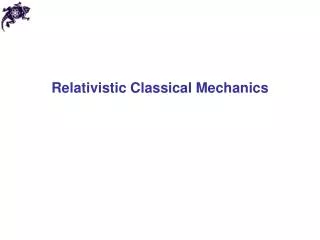
Relativistic Classical Mechanics. Albert Abraham Michelson (1852 – 1931). Edward Williams Morley (1838 – 1923). James Clerk Maxwell (1831-1879). XIX century crisis in physics: some facts Maxwell : equations of electromagnetism are not invariant under Galilean transformations

E N D
Albert Abraham Michelson (1852 – 1931) Edward Williams Morley (1838 – 1923) James Clerk Maxwell (1831-1879) • XIX century crisis in physics: • some facts • Maxwell: equations of electromagnetism are not invariant under Galilean transformations • Michelson and Morley: the speed of light is the same in all inertial systems
7.1 • Postulates of the special theory • 1) The laws of physics are the same to all inertial observers • 2) The speed of light is the same to all inertial observers • Formulation of physics that explicitly incorporates these two postulates is called covariant • The space and time comprise a single entity: spacetieme • A point in spacetime is called event • Metric of spacetime is non-Euclidean
7.5 • Tensors • Tensor of rank n is a collection of elements grouped through a set of n indices • Scalar is a tensor of rank 0 • Vector is a tensor of rank 1 • Matrix is a tensor of rank 2 • Etc. • Tensor product of two tensors of ranks m and n is a tensor of rank (m + n) • Sum over a coincidental index in a tensor product of two tensors of ranks m and n is a tensor of rank (m + + n – 2)
7.5 • Tensors • Tensor product of two vectors is a matrix • Sum over a coincidental index in a tensor product of two tensors of ranks 1 and 1 (two vectors) is a tensor of rank 1 + 1 – 2 = 0 (scalar): scalar product of two vectors • Sum over a coincidental index in a tensor product of two tensors of ranks 2 and 1 (a matrix and a vector) is a tensor of rank 2 + 1 – 2 = 1 (vector) • Sum over a coincidental index in a tensor product of two tensors of ranks 2 and 2 (two matrices) is a tensor of rank 2 + 2 – 2 = 2 (matrix)
7.4 7.5 • Metrics, covariant and contravariant vectors • Vectors, which describe physical quantities, are called contravariantvectors and are marked with superscripts instead of a subscripts • For a given space of dimension N, we introduce a concept of a metric – N x N matrix uniquely defining the symmetry of the space (marked with subscripts) • Sum over a coincidental index in a product of a metric and a contravariant vecor is a covariantvector or a 1-form (marked with subscripts) • Magnitude: square root of the scalar product of a contravariant vector and its covariant counterpart
7.4 7.5 • 3D Euclidian Cartesian coordinates • Contravariant infinitesimal coordinate vector: • Metric • Covariant infinitesimal coordinate vector: • Magnitude:
7.4 7.5 • 3D Euclidian spherical coordinates • Contravariant infinitesimal coordinate vector: • Metric • Covariant infinitesimal coordinate vector: • Magnitude:
7.4 7.5 David Hilbert (1862 – 1943) • Hilbert space of quantum-mechanical wavefunctions • Contravariant vector (ket): • Covariant vector (bra): • Magnitude: • Metric:
7.4 7.5 • 4D spacetime • Contravariant infinitesimal coordinate 4-vector: • Metric • Covariant infinitesimal coordinate vector:
7.4 7.5 • 4D spacetime • Magnitude: • This magnitude is called differential interval • Interval (magnitude of a 4-vector connecting two events in spacetime): • Interval should be the same in all inertial reference frames • The simplest set of transformations that preserve the invariance of the interval relative to a transition from one inertial reference frame to another: Lorentz transformations
7.2 Hendrik Antoon Lorentz (1853 – 1928) • Lorentz transformations • We consider two inertial reference frames S and S’; relative velocity as measured in S is v : • Then Lorentz transformations are: • Lorentz transformations can be written in a • matrix form
7.2 Lorentz transformations
7.2 • Lorentz transformations • If the reference frame S‘ moves parallel to the x axis of the reference frame S: • If two events happen at the same location in S: • Time dilation
7.2 • Lorentz transformations • If the reference frame S‘ moves parallel to the x axis of the reference frame S: • If two events happen at the same time in S: • Length contraction
7.3 • Velocity addition • If the reference frame S‘ moves parallel to the x axis of the reference frame S: • If the reference frame S‘‘ moves parallel to the x axis of the reference frame S‘:
7.3 • Velocity addition • The Lorentz transformation from the reference frame S to the reference frame S‘‘: • On the other hand:
7.4 • Four-velocity • Proper time is time measured in the system where the clock is at rest • For an object moving relative to a laboratory system, we define a contravariant vector of four-velocity:
7.4 • Four-velocity • Magnitude of four-velocity
7.1 t t’ Hermann Minkowski (1864 - 1909) x’ x • Minkowski spacetime • Lorentz transformations for parallel axes: • How do x’ and t’ axes look in • the x and t axes? • t’ axis: • x’ axis:
7.1 t x • Minkowski spacetime • When • How do x’ and t’ axes look in • the x and t axes? • t’ axis: • x’ axis:
7.1 t t’ x’ x • Minkowski spacetime • Let us synchronize the clocks of the S and S’ frames at the origin • Let us consider an event • In the S frame, the event is • to the right of the origin • In the S‘ frame, the event is • to the left of the origin
7.1 t t’ x’ x • Minkowski spacetime • Let us synchronize the clocks of the S and S’ frames at the origin • Let us consider an event • In the S frame, the event is • after the synchronization • In the S‘ frame, the event is • before the synchronization
7.1 Minkowski spacetime
7.4 • Four-momentum • For an object moving relative to a laboratory system, we define a contravariant vector of four-momentum: • Magnitude of four-momentum
7.4 • Four-momentum • Rest-mass: mass measured in the system where the object is at rest • For a moving object: • The equation has units of energy squared • If the object is at rest
7.4 Four-momentum
7.4 • Four-momentum • Rest-mass energy: energy of a free object at rest – an essentially relativistic result • For slow objects: • For free relativistic objects, we introduce therefore the kinetic energy as
7.9 • Non-covariant Lagrangian formulation of relativistic mechanics • As a starting point, we will try to find a non-covariant Lagrangian formulation (the time variable is still separate) • The equations of motion should look like
7.9 • Non-covariant Lagrangian formulation of relativistic mechanics • For an electromagnetic potential, the Lagrangian is similar • The equations of motion should look like • Recall our derivations in “Lagrangian Formalism”:
7.9 • Non-covariant Lagrangian formulation of relativistic mechanics • Example: 1D relativistic motion in a linear potential • The equations of motion: • Acceleration is hyperbolic, not parabolic
7.9 8.4 • Non-covariant Hamiltonian formulation of relativistic mechanics • We start with a non-covariant Lagrangian: • Applying a standard procedure • Hamiltonian equals the total energy of the object
7.9 8.4 • Non-covariant Hamiltonian formulation of relativistic mechanics • We have to express the Hamiltonian as a function of momenta and coordinates:
More on symmetries • Full time derivative of a Lagrangian: • Form the Euler-Lagrange equations: • If
7.9 8.4 • Non-covariant Hamiltonian formulation of relativistic mechanics • Example: 1D relativistic harmonic oscillator • The Lagrangian is not an explicit function of time • The quadrature involves elliptic integrals
7.10 • Covariant Lagrangian formulation of relativistic mechanics: plan A • So far, our canonical formulations were not Lorentz-invariant – all the relationships were derived in a specific inertial reference frame • We have to incorporate the time variable as one of the coordinates of the spacetime • We need to introduce an invariant parameter, describing the progress of the system in configuration space: • Then
7.10 • Covariant Lagrangian formulation of relativistic mechanics: plan A • Equations of motion • We need to find Lagrangians producing equations of motion for the observable behavior • First approach: use previously found Lagrangians and replace time and velocities according to the rule:
7.10 • Covariant Lagrangian formulation of relativistic mechanics: plan A • Then • So, we can assume that • Attention: regardless of the functional dependence, the new Lagrangian is a homogeneous function of the generalized velocities in the first degree:
7.10 • Covariant Lagrangian formulation of relativistic mechanics: plan A • From Euler’s theorem on homogeneous functions it follows that • Let us consider the following sum
7.10 • Covariant Lagrangian formulation of relativistic mechanics: plan A • If three out of four equations of motion are satisfied, the fourth one is satisfied automatically
7.10 • Example: a free particle • We start with a non-covariant Lagrangian
7.10 • Example: a free particle • Equations of motion
7.10 • Example: a free particle • Equations of motion of a free relativistic particle
7.10 • Covariant Lagrangian formulation of relativistic mechanics: plan B • Instead of an arbitrary invariant parameter, we can use proper time • However • Thus, components of the four-velocity are not independent: they belong to three-dimensional manifold (hypersphere) in a 4D space • Therefore, such Lagrangian formulation has an inherent constraint • We will impose this constraint only after obtaining the equations of motion
7.10 • Covariant Lagrangian formulation of relativistic mechanics: plan B • In this case, the equations of motion will look like • But now the Lagrangian does not have to be a homogeneous function to the first degree • Thus, we obtain freedom of choosing Lagrangians from a much broader class of functions that produce Lorentz-invariant equations of motion • E.g., for a free particle we could choose
7.10 • Covariant Lagrangian formulation of relativistic mechanics: plan B • If the particle is not free, then interaction terms have to be added to the Lagrangian – these terms must generate Lorentz-invariant equations of motion • In general, these additional terms will represent interaction of a particle with some external field • The specific form of the interaction will depend on the covariant formulation of the field theory • Such program has been carried out for the following fields: electromagnetic, strong/weak nuclear, and a weak gravitational
7.10 • Covariant Lagrangian formulation of relativistic mechanics: plan B • Example: 1D relativistic motion in a linear potential • In a specific inertial frame, the non-covariant Lagrangian was earlier shown to be • The covariant form of this problem is • In a specific inertial frame, the interaction vector will be reduced to
7.10 7.6 • Example: relativistic particle in an electromagnetic field • For an electromagnetic field, the covariant Lagrangian has the following form: • The corresponding equations of motion:
7.10 7.6 • Example: relativistic particle in an electromagnetic field • Maxwell's equations follow from this covariant formulation (check with your E&M class)