Download

1 / 46
460 likes | 665 Views
Models for Non-Stationary Time Series. The ARIMA( p,d,q ) time series. The ARIMA( p,d,q ) time series. Many non-stationary time series can be converted to a stationary time series by taking d th order differences. Let { x t |t T } denote a time series such that

E N D
Models for Non-Stationary Time Series The ARIMA(p,d,q) time series
The ARIMA(p,d,q) time series Many non-stationary time series can be converted to a stationary time series by taking dth order differences.
Let {xt|t T} denote a time series such that {wt|t T} is an ARMA(p,q) time series where wt= Ddxt = (I – B)dxt = the dth order differences of the series xt. Then {xt|t T} is called an ARIMA(p,d,q) time series (an integrated auto-regressive moving average time series.)
The equation for the time series {wt|t T} is: b(B)wt = d+ a(B)ut The equation for the time series {xt|t T} is: b(B)Ddxt = d+ a(B)ut or f(B)xt =d+ a(B)ut.. Where f(B) =b(B)Dd =b(B)(I - B) d
Suppose that d roots of the polynomialf(x)are equal to unity thenf(x) can be written: f(B)= (1 -b1x - b2x2-... -bpxp)(1-x)d. and f(B) could be written: f(B) = (I -b1B - b2B2 -... -bpBp)(I-B)d= b(B)Dd. In this case the equation for the time series becomes: f(B)xt = d+ a(B)ut or b(B)Ddxt =d+ a(B)ut..
Comments: • The operator f(B) =b(B)Dd= 1 -f1x-f2x2 -... - fp+dxp+d is called the generalized autoregressive operator. (d roots are equal to 1, the remaining p roots have |ri| > 1) 2.The operatorb(B) is called the autoregressive operator. (p roots with |ri| > 1) 3.The operatora(B) is called moving average operator.
Example – ARIMA(1,1,1) The equation: (I – b1B)(I – B)xt = d+ (I + a1)ut (I – (1 + b1) B+b1B2)xt = d+ ut + a1 ut - 1 xt – (1 + b1) xt-1+b1xt-2 = d+ ut + a1 ut – 1 or xt= (1 + b1) xt-1–b1xt-2+d+ ut + a1 ut – 1
If a time series, {xt: t T},that is seasonal we would expect observations in the same season in adjacent years to have a higher auto correlation than observations that are close in time (but in different seasons. For example for data that is monthly we would expect the autocorrelation function to look like this
The AR(1) seasonal model This model satisfies the equation: The autocorrelation for this model can be shown to be: This model is also an AR(12) model with b1 = … = b11 = 0
The AR model with both seasonal and serial correlation This model satisfies the equation: This model is also an AR(13) model. The autocorrelation for this model will satisfy the equations:
The Difference equation Form: xt =f1xt-1 + f2xt-2+... +fp+dxt-p-d + d + ut +a1ut-1+ a2ut-2+...+ aqut-q • b(B)Ddxt = d+a(B)ut
The Random Shock Form: xt =m(t) + ut+y1ut-1 + y2ut-2 +y3ut-3 +... xt=m(t) +y(B)ut
The Inverted Form: xt =p1xt-1 +p2xt-2 +p3xt-3+ ...+ t + ut p(B)xt =t+ ut
Example Consider the ARIMA(1,1,1) time series (I – 0.8B)Dxt= (I + 0.6B)ut (I – 0.8B) (I –B) xt= (I + 0.6B)ut (I – 1.8B + 0.8B2) xt= (I + 0.6B)ut xt = 1.8 xt - 1 - 0.8 xt - 2 + ut+ 0.6ut -1 Difference equation form
The random shock form (I – 1.8B + 0.8B2) xt= (I + 0.6B)ut xt= (I – 1.8B + 0.8B2)-1(I + 0.6B)ut xt= (I + 2.4B + 3.52B2 + 4.416B3 + 5.1328B4 + … )ut xt= ut+ 2.4 ut - 1 + 3.52 ut - 2 + 4.416 ut - 3+ 5.1328 ut - 4+ …
The Inverted form (I – 1.8B + 0.8B2) xt= (I + 0.6B)ut (I + 0.6B)-1(I – 1.8B + 0.8B2)xt= ut (I - 2.4B + 2.24B2 – 1.344 B3 + 0.8064B4 +… )xt= ut xt= 2.4 xt - 1 - 2.24 xt - 2 + 1.344 xt - 3- 0.8064 xt - 4+ … +ut
Forecasting an ARIMA(p,d,q) Time Series • Let PT denote {…, xT-2, xT-1, xT} = the “past” until time T. • Then the optimal forecast of xT+l given PT is denoted by: • This forecast minimizes the mean square error
Three different forms of the forecast • Random Shock Form • Inverted Form • Difference Equation Form Note:
Random Shock Form of the forecast xt =m(t)+ ut+y1ut-1+y2ut-2 +y3ut-3 +... Recall or xT+l =m(T + l)+uT+l +y1uT+l-1 +y2uT+l-2+y3uT+l-3+... Taking expectations of both sides and using
Note: xt =m(t) +ut +y1ut-1+y2ut-2+y3ut-3+... To compute this forecast we need to compute {…, uT-2, uT-1, uT} from {…, xT-2, xT-1, xT}. Thus and Which can be calculated recursively
The Error in the forecast: The Mean Sqare Error in the Forecast Hence
Prediction Limits for forecasts (1 – a)100% confidence limits for xT+l
The Inverted Form: p(B)xt =t+ utor xt =p1xt-1+p2xt-2+p3x3+ ... + t + ut where p(B) = [a(B)]-1f(B)=[a(B)]-1[b(B)Dd] = I -p1B -p2B2-p3B3-...
The Inverted form of the forecast Note: xt =p1xt-1 +p2xt-2 +... +t+ ut and for t = T+l xT+l = p1xT+l-1+p2xT+l-2+...+t + uT+l Taking conditional Expectations
The Difference equation form of the forecast xT+l =f1xT+l-1+f2xT+l-2+ ...+ fp+dxT+l-p-d + d+ uT+l +a1uT+l-1+a2uT+l-2+... + aquT+l-q Taking conditional Expectations
Example: ARIMA(1,1,2) The Model: xt - xt-1 = b1(xt-1 - xt-2) + ut +a1ut + a2ut or xt = (1 + b1)xt-1 - b1xt-2 + ut+ a1ut + a2ut or f(B)xt = b(B)(I-B)xt = a(B)ut where f(x) = 1 - (1 + b1)x + b1x2 = (1 - b1x)(1-x) and a(x) = 1 + a1x + a2x2 .
The Random Shock form of the model: xt =y(B)ut where y(B) = [b(B)(I-B)]-1a(B) = [y(B)]-1a(B) i.e. y(B) [f(B)] = a(B). Thus (I + y1B + y2B2 + y3B3 + y4B4 + ... )(I - (1 + b1)B + b1B2) = I + a1B + a2B2 Hence a1 = y1 - (1 + b1) or y1 = 1 + a1 + b1. a2 = y2 - y1(1 + b1) + b1 or y2 =y1(1 + b1) - b1 + a2. 0 = yh - yh-1(1 + b1) + yh-2b1 or yh = yh-1(1 + b1) - yh-2b1 for h ≥ 3.
The Inverted form of the model: p(B)xt = ut where p(B) = [a(B)]-1b(B)(I-B) = [a(B)]-1f(B) i.e. p(B) [a(B)] = f(B). Thus (I - p1B - p2B2 - p3B3 - p4B4 - ... )(I + a1B + a2B2) = I - (1 + b1)B + b1B2 Hence -(1 + b1) = a1 - p1 or p1 = 1 + a1 + b1. b1 = -p2 - p1a1 + a2 or p2 = -p1a1 - b1 +a2. 0 = -ph - ph-1a1 - ph-2a2 or ph= -(ph-1a1 + ph-2a2) for h ≥ 3.
Now suppose that b1 = 0.80, a1 = 0.60 and a2 = 0.40 then the Random Shock Form coefficients and the Inverted Form coefficients can easily be computed and are tabled below:
Computation of the Random Shock Series, One-step Forecasts One-step Forecasts Random Shock Computations
Computation of the Mean Square Error of the Forecasts and Prediction Limits Mean Square Error of the Forecasts Prediction Limits
Raw Observations, One-step Ahead Forecasts, Estimated error , Error