Download
1 / 36
360 likes | 545 Views
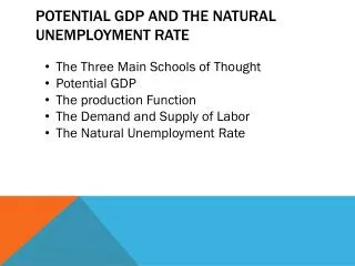
24. Potential GDP and the Natural Unemployment Rate. CHAPTER. C H A P T E R C H E C K L I S T. When you have completed your study of this chapter, you will be able to. 1 Explain the forces that determine potential GDP and the real wage rate and employment at full employment.

E N D
24 Potential GDP and the Natural Unemployment Rate CHAPTER
C H A P T E R C H E C K L I S T When you have completed your study of this chapter, you will be able to • 1Explain the forces that determine potential GDP and the real wage rate and employment at full employment. • 2 Explain the forces that determine the natural unemployment rate.
MACROECONOMIC APPROACHES AND PATHWAYS • The Two Main Schools of Thought The two main approaches to macroeconomics are based on two schools of thought: • Classical macroeconomics • Keynesian macroeconomics
MACROECONOMIC APPROACHES AND PATHWAYS MACROECONOMIC APPROACHES AND PATHWAYS • Classical macroeconomics is a body of theory about how a market economy works and why it experiences economic growth and fluctuations. • The classical view is that markets work well and deliver the best available macroeconomic performance. • The economy will fluctuate, and growth will slow down from time to time. • But no government remedy can improve the performance of the market.
MACROECONOMIC APPROACHES AND PATHWAYS MACROECONOMIC APPROACHES AND PATHWAYS • Classical macroeconomic fell into disrepute during the 1930s, which was a decade of high unemployment and stagnant production throughout the world. • Great Depression is a decade (the 1930s) of high unemployment and stagnant production throughout the world economy. • Classical macroeconomics predicted that the Great Depression would end but gave no method for ending it more quickly.
MACROECONOMIC APPROACHES AND PATHWAYS • Keynesian macroeconomics is a body of theory about how a market economy works that stresses it inherent instability and the need for active government intervention to achieve full employment and sustained economic growth. • John Maynard Keynes, in his book “The General Theory of Employment, Interest, and Money,” began this school of thought. • Keynes’ theory was that too little consumer spending and investment lead to the Great Depression.
MACROECONOMIC APPROACHES AND PATHWAYS • Keynes’ solution to depression and high unemployment was increased government spending. • But Keynes predicted that his policy aimed at curing unemployment in the short term might increase it in the long term. • This prediction became reality during the 1960s and 1970s, when inflation exploded, growth slowed, and unemployment increased. • It was time for another challenge to the mainstream: new macroeconomics
MACROECONOMIC APPROACHES AND PATHWAYS • The New Macroeconomics • New macroeconomics is a body of theory about how a market economy works based on the view that macro outcomes depend on micro choices—the choices of rational individuals and firms interacting in markets. • New classical macroeconomics incorporates the ideas of classical economists that markets work and new Keynesian macroeconomics incorporates the ideas of Keynesian economists that markets adjust slowly.
MACROECONOMIC APPROACHES AND PATHWAYS • The key difference between the two new schools is in their view of how quickly price and wages adjust in the face of excess demand or excess supply. • But this difference is tiny, and a consensus is emerging. • The Road Ahead • We follow the new consensus and begin with an explanation of what determines real GDP and employment and the pace of economic growth.
24.1 POTENTIAL GDP • Potential GDP is the level of real GDP that the economy would produce if it were at full employment. • We produce the goods and services that make up real GDP by using factors of production: labor and human capital, physical capital, land, and entrepreneurship. • At any given time, the quantities of human capital, physical capital, land, entrepreneurship, and the state of technology are fixed.
24.1 POTENTIAL GDP • The quantity of labor employed depends on the choices of people and businesses. • So real GDP produced depend on the quantity of labor employed. • To describe the relationship between real GDP and the quantity of labor employed, we use a relationship called the production function.
24.1 POTENTIAL GDP • The Production Function • Production function is a relationship that shows the maximum quantity of real GDP that can be produced as the quantity of labor employed changes and all other influences on production remain the same.
24.1 POTENTIAL GDP • Figure 24.1 shows the production function. • 100 billion hours of labor can produce $6 trillion of real GDP at point A.
24.1 POTENTIAL GDP • 200 billion hours of labor can produce $10 trillion of real GDP at point B. • 300 billion hours of labor can produce $12 trillion of real GDP at point C. • The production function PF is a limit to what is attainable.
24.1 POTENTIAL GDP • The production function is a boundary between the attainable and the unattainable. • The production function displays diminishing returns: The tendency for each additional hour of labor employed to produce successively smaller additional amounts of real GDP.
24.1 POTENTIAL GDP • The Labor Market • The Demand for Labor • Quantity of labor demanded is the total labor hours that all the firms in the economy plan to hire during a given time period at a given real wage rate.
24.1 POTENTIAL GDP • Demand for labor is the relationship between the quantity of labor demanded and real wage rate when all other influences on firms’ hiring plans remain the same. • The lower the real wage rate, the greater is the quantity of labor demanded.
24.1 POTENTIAL GDP • Figure 24.2 shows the demand for labor.
24.1 POTENTIAL GDP • The Supply of Labor • Quantity of labor supplied is the number of labor hours that all the households in the economy plan to work during a given time period and at a given real wage rate. • Supply of labor is the relationship between the quantity of labor supplied and the real wage rate when all other influences on work plans remain the same.
24.1 POTENTIAL GDP • Figure 24.3 shows the supply of labor.
24.1 POTENTIAL GDP • The quantity of labor supplied increases as the real wage rate increases for two reasons: • Hours per person increase as the real wage rate increases. • The labor force participation rate increases as the real wage rate increases.
24.1 POTENTIAL GDP • Labor Market Equilibrium • A rise in the real wage rate eliminates a shortage of labor by decreasing the quantity demanded and increasing the quantity supplied. • A fall in the real wage rate eliminates a surplus of labor by increasing the quantity demanded and decreasing the quantity supplied. • If there is neither a shortage nor a surplus, the labor market is in equilibrium.
24.1 POTENTIAL GDP • Figure 24.4(a) shows labor market equilibrium. 1. Full employment occurs when the quantity of labor demanded equals the quantity of labor supplied. 2. Equilibrium real wage rate is $30 an hour. 3. Full-employment quantity of labor is 200 billion hours a year.
24.1 POTENTIAL GDP • Full Employment and Potential GDP • When the labor market is in equilibrium, the economy is at full employment. • When the economy is at full employment, real GDP equals potential GDP.
24.1 POTENTIAL GDP • Figure 24.4(b) shows potential GDP. 1. When the full-employment quantity of labor is 200 billion hours a year, 2. Potential GDP is $10 billion.
24.2 THE NATURAL UNEMPLOYMENT RATE • So far, we’ve focused on the forces that determine the quantity of labor employed. • Now we look at what determine the unemployment rate when the economy is at full employment? • To understand the amount of frictional and structural unemployment that exists at the natural unemployment rate, economists focus on two fundamental causes of unemployment: • Job search • Job rationing
24.2 THE NATURAL UNEMPLOYMENT RATE • Job Search • Job search is the activity of looking for an acceptable vacant job. • The amount of job search depends on • Demographic change • Unemployment benefits • Structural change
24.2 THE NATURAL UNEMPLOYMENT RATE • Demographic Change • An increase in the proportion of the population that is of working age brings an increase in the entry rate into the labor force and an increase in the unemployment rate. • This factor increased the unemployment rate during the 1970s and decreased it during the 1980s.
24.2 THE NATURAL UNEMPLOYMENT RATE • Unemployment Benefits • An unemployed person who receives no unemployment benefits faces a high opportunity cost of job search and has an incentive to keep job search brief. • An unemployed person who receives generous unemployment benefits faces a lower opportunity cost of job search and has an incentive to search for longer.
24.2 THE NATURAL UNEMPLOYMENT RATE • Structural Change • Labor market flows and unemployment are influenced by the pace and direction of technological change. • Technological change can bring a structural slump, as it did during the 1970s. • Technological change can bring a structural boom, as it did during the 1990s.
24.2 THE NATURAL UNEMPLOYMENT RATE • Job Rationing • Job rationing is a situation that arises when the real wage rate is above the equilibrium level. • The real wage rate might be set above the equilibrium level for three reasons: • Efficiency wage • Minimum wage • Union wage
24.2 THE NATURAL UNEMPLOYMENT RATE • Efficiency Wage • If a firm pays only the going market wage, employees have no incentive to work hard because they know that even if they are fired for shirking, they can find another job at a similar wage rate. • So some firms pay an efficiency wage. • Efficiency wage is a real wage rate that is set above the full-employment equilibrium wage rate to induce greater work effort.
24.2 THE NATURAL UNEMPLOYMENT RATE • The Minimum Wage • If the government sets a minimum wage above the equilibrium wage rate, unemployment results. • Union Wage • Labor unions operate in some labor markets and agree a wage with employers. • Union wage is a wage rate that results from collective bargaining between a labor union and a firm.
24.2 THE NATURAL UNEMPLOYMENT RATE • Job Rationing and Unemployment • The above-equilibrium real wage rate decreases the quantity of labor demanded and increases the quantity of labor supplied. • If the real wage rate is above the full-employment equilibrium level, the natural unemployment rate increases.
24.2 THE NATURAL UNEMPLOYMENT RATE • Figure 24.5 shows how job rationing increases the natural unemployment rate. • An efficiency wage rate • 1. Decreases the quantity demanded—job rationing. 2. Increases the quantity of labor supplied. 3. Increases the natural unemployment rate.