Download
1 / 10
100 likes | 379 Views
Discrete Mathematics Math 6A. Instructor: M. Welling. 1.1 Propositions. Logic allows consistent mathematical reasoning. Many applications in CS: construction and verification computer programs, circuit design, etc.

E N D
Discrete MathematicsMath 6A Instructor: M. Welling
1.1 Propositions • Logic allows consistent mathematical reasoning. • Many applications in CS: construction and verification computer programs, • circuit design, etc. Proposition:A statement that is either true (T) or false (F). example: Toronto is the capital of Canada in 2003 (F). 1+1=2 (T). counter-example: I love this class. Compound Propositions:New propositions formed by existing propositions and logical operators. Let “P” be a proposition. Then (“NOT P”) is another one stating that: It is not the case that “P”.
1.1 Propositions truth table example: P: Today is Tuesday. NOT P: Today is not Tuesday. NOT is the negation operator. Another class of operators are the “connectives”. P AND Q conjunction P OR Q disjunction , inclusive OR. P XOR Q exclusive OR. example: Bob is married to Carol. (T) Bob is married to Betty or to Carol. (T) Bob is married to Betty and to Carol (F).
1.1 Implications Implication : P Q , P IMPLIES Q. P is hypothesis, Q is consequence. some names: if P then Q, Q when P, Q follows from P, P only if Q. example: If you make no mistakes, then you’ll get an A. Bidirectional implication: PQ , P if and only if (iff) Q. Implications are often used in mathematical proofs. Consider: P Q. converse: Q P. contra-positive: (NOT Q) (NOT P) (equiv.) inverse: (NOT P) (NOT Q). weird?
1.1 Precedence, Bits. Order of precedence: NOT, AND, OR, XOR, , . example: PQ AND NOT R = P (Q AND (NOT R) ). Bits are units of information. 1=T, 0=F. Bit-strings are sequences of bits: 00011100101010 We can use our logic operators to manipulate these bit-strings: example: 0110 AND 1100 = 0100 puzzle: Is this a proposition: “This statement is false”? if S = T S = F, if S = F S = T whoa: it is neither true nor false!
1.2 Propositional Equivalences Tautology:Proposition that is always true. for example: P OR (NOT P). Contradiction:Proposition that is always false. for example:P AND (NOT P). Others: Contingencies. Two propositions are logically equivalent if P Q is always true (tautology). This is denoted by . Example: Morgan’s Law:
1.2 Propositional Equivalences Proving equivalences by truth tables can easily become computationally demanding: equivalence with 1 prop.: truth table has columns of size 2. equivalence with 2 prop.: ..................................................4. equivalence with 3 prop.: ..................................................8. equivalence with n prop.: ................................................... (How many times do we need to fold the NY-times to fit between the earth and the moon ?) Solution: we use a list of known logical equivalences (building blocks) and manipulate the expression. See page 24 for a list of equivalences.
1.3 Predicates & Quantification Let’s consider statements with variables: x > 3. x is the subject. >3 is the predicate or property of the subject. We introduce a propositional function, P(x), that denotes >3. If X has is a specific number, the function becomes a proposition (T or F). example: P(2) = F, P(4) = T. More generally, we can have “functions” of more than one variable. For each input value it assigns either T or F. example: Q(x,y) = ( x=y+3 ). Q(1,2) = ( 1=2+3 ) = F Q(3,0) =( 3=0+3)=T
1.3 Predicates and Quantification We do not always have to insert specific values. We can make propositions for general values in a domain (or universe of discourse): This is called: quantification. Universal Quantification: P(x) is true for all values of x in the domain: Existential Quantification: There exists an element x in the domain such that P(x) is true: example: domain x is real numbers. P(x) is x > -1. (F : counter-example: x=-2) (T) example: domain is positive real numbers, P(x) is x>-1. (T) (T)
1.3 Binding & negations A variable is bound if it has a value or a quantifier is “acting” on it. A statement can only become a proposition if all variables are bound. example: x is bound, y is free. The scope of a quantifier is the part of the statement on which it is acting. example: scope x scope y We can also negate propositions with quantifiers. Two important equivalences: It is not the case that for all x P(x) is true = there must be an x for which P(x) is not true It is not true that there exists an x for which P(x) is true = P(x) must be false for all x