Download
1 / 45
450 likes | 601 Views
Numerical studies of the ABJM theory for arbitrary N at arbitrary coupling constant. Masazumi Honda. SOKENDAI & KEK . Reference: JHEP 0312 164(2012) (arXiv:1202.5300 [ hep-th ]). In collaboration with Masanori Hanada (KEK), Yoshinori Honma (SOKENDAI & KEK),

E N D
Numerical studies of the ABJM theoryfor arbitrary N at arbitrary coupling constant Masazumi Honda SOKENDAI & KEK Reference: JHEP 0312 164(2012) (arXiv:1202.5300 [hep-th]) In collaboration with Masanori Hanada (KEK), Yoshinori Honma (SOKENDAI & KEK), Jun Nishimura (SOKENDAI & KEK), ShotaroShiba (KEK) & Yutaka Yoshida (KEK) 名古屋大弦理論セミナー 2012年4月23日
Introduction F (free energy) N3/2 Surprisingly, we can realize this result even by our laptop
Numerical simulation of U(N)×U(N) ABJM on S3 Motivation: ( k: Chern-Simons level ) CFT3 AdS4 / relatively easy ABJM theory (Intermediate) Extremely difficult! Key for a relation between string and M-theory? [Aharony-Bergman-Jafferis-Maldacena ’08] relatively hard Investigate the whole region by numerical simulation!
This talk is about… Monte Carlo calculation of the Free energy in U(N)×U(N) ABJM theory on S3(with keeping all symmetry) ・Test all known analytical results ・Relation between the known results and our simulation result
Developments on ABJM Free energy ・June 2008: ABJM was born. [Aharony-Bergman-Jafferis-Maldacena] ・July 2010: Planar limit for strong coupling [Drukker-Marino-Putrov] Agrees with SUGRA’s result!! [Cf. Cagnazzo-Sorokin-Wulff ’09] ※CP3 has nontrivial 2-cycle ~string wrapped on CP1⊂ CP3=worldsheetinstanton? ・November 2010: Calculation for k=fixed, N→∞ [Herzog-Klebanov-Pufu-Tesileanu] Formally same (※ λ=N/k)
(Cont’d)Development on ABJM free energy ・June 2011:Summing up all genus around planar limit for strong λ [Fuji-Hirano-Moriyama] Formally same ・October 2011: Exact calculation for N=2 [Okuyama] ・October 2011: Calculation for k<<1, k<<N [Marino-Putrov] where Correction to Airy function →How about for large k?? ・February 2012: Numerical simulation in the whole region(=this talk) [ Hanada-M.H.-Honma-Nishimura-Shiba-Yoshida] At least up to instanton effect,for all k, Free energy is a smooth function of k !!
Contents Introduction & Motivation 2. How to put ABJM on a computer 3. Result 4. Interpretation 5. Summary & Outlook
How do we ABJM on a computer? ~Approach by the orthodox method(=Lattice)~ Action: Difficulties in “formulation” ・It is not easy to construct CS term on a lattice ・It is generally difficult to treat SUSY on a lattice [Cf. Bietenholz-Nishimura ’00] [Cf. Giedt ’09] Practical difficulties ・∃Many fermionicdegrees of freedom → Heavy computational costs ・CS term = purely imaginary → sign problem hopeless…
(Cont’d)How do we put ABJM on a computer? Lattice approach is hopeless… We can apply the localization method for the ABJM partition function
Localization method Original partition function: [Cf. Pestun ’08] where 1 parameter deformation: Consider t-derivative: Assuming Q is unbroken We can use saddle point method!!
(Cont’d) Localization method Consider fluctuation around saddle points: where
Localization of ABJM theory [Kapustin-Willet-Yaakov ’09]
(Cont’d) Localization of ABJM theory Saddle point: Gauge 1-loop CS term Matter 1-loop
(Cont’d)How do we put ABJM on a computer? After applying the localization method, the partition function becomes just 2N-dimentional integration: Sign problem Further simplification occurs!!
Simplification of ABJM matrix model [Kapustin-Willett-Yaakov ’10, Okuyama ‘11, Marino-Putrov ‘11] Cauchy identity: Fourier trans.:
(Cont’d) Simplification of ABJM matrix model Gaussian integration Fourier trans.: Cauchy id.:
Short summary Lattice approach is hopeless… (∵SUSY, sign problem, etc) Localization method Complex ≠probability Cauchy identity, Fourier trans. & Gauss integration Easy to perform simulation even by our laptop
How to calculate the free energy Problem: Monte Carlo can calculate only expectation value We regard the partition function as an expectation value under another ensemble: VEV under the action: Note:
Contents Introduction & Motivation 2. How to put ABJM on a computer 3. Result 4. Interpretation 5. Summary & Outlook
Warming up: Free energy for N=2 There is the exact result for N=2: [ Okuyama ’11] for odd k for even k F (free energy) Complete agreement with the exact result !! k ( CS level )
Result for Planar limit [Drukker-Marino-Putrov ’10] ・Weak couling: ・Strong coupling: Worldsheetinstanton Weak coupling Different from worldsheetinstanton behavior Strong coupling strong weak strong weak
3/2 power low in 11d SUGRA limit [Drukker-Marino-Putrov ‘10, Herzog-Klebanov-Pufu-Tesileanu ‘10] 11d classical SUGRA: F/N3/2 F N3/2 1/N
(Cont’d) 3/2 power low in 11d SUGRA limit 11d classical SUGRA: Perfect agreement !!
Comparison with Fuji-Hirano-Moriyama [Fuji-Hirano-Moriyama ’11] Ex.) For N=4 Weak coupling FHM Discrepancy independent of N and dependent on k →different from instantonbahavior (~exp dumped) Almost agrees with FHM for strong coupling →more precise comparison by taking difference Almost agrees with FHM for strong coupling →more precise comparison by taking difference strong weak
Contents Introduction & Motivation 2. How to put ABJM on a computer 3. Result 4. Interpretation 5. Summary & Outlook
Fermi gas approach [Marino-Putrov ’11] Cauchy id.: Regard as a Fermi gas system Result: where Our result says that this remains even for large k??
Origin of Discrepancy for the Planar limit (without MC) [Marino-Putrov ‘10] Analytic continuation: [Cf. Yost ’91, Dijkgraaf-Vafa ‘03] Lens space L(2,1)=S3/Z2matrix model: Genus expansion:
(Cont’d))Origin of Discrepancy for the Planar limit (without MC) [Drukker-Marino-Putrov ‘10] The “derivative” of planar free energy is exactly found as We impose the boundary condition: Cf. By using asymptotic behavior, Necessary for satisfying b.c. , taken as 0 for previous works
Origin of discrepancy for all genus Discrepancy is fitted by This is explained by ``constant map’’contribution in language of topological string: [ Bershadsky-Cecotti-Ooguri-Vafa ’93,Faber-Pandharipande ’98, Marino-Pasquwtti-Putrov ’09 ] Divergent, but Borelsummable:
Comparison with discrepancy and Fermi gas Divergent, but Borelsummable: genus 2 Borel sum of Constant map realizes FermiGas(small k)result!! →Can we understand the relation analytically? Fermi Gas
Fermi Gas from Constant map Constant map contribution: Borel Expand around k=0 True for all k? All order form? Agrees with Fermi Gas result! →Fermi Gas result is asymptotic series around k=0
Contents Introduction & Motivation 2. How to put ABJM on a computer 3. Result 4. Interpretation 5. Summary & Outlook
Summary Monte Carlo calculation of the Free energy in U(N)×U(N) ABJM theory on S3(with keeping all symmetry) ・Discrepancy from Fuji-Hirano-Moriyama not originated by instantons is explained by constant map contribution ・Although summing up all genus constant map is asymptotic series, it is Borelsummable. ・The free energy for whole region up to instanton effect: ~instanton effect where ・Predict all order form of Fermi Gas result:
Problem ・What is a physical meaning of constant map contribution? - In Fermi gas description, this is total energy of membrane instanton [ Becker-Becker-Strominger ‘95] - Why is ABJM related to the topological string theory? ・If there is also constant map contribution on the gravity side, there are α’-corrections at every order of genus - Does it contradict with the proof for non-α’-correction? [ Kallosh-Rajaraman ’98] - Is constant map origin of free energy on the gravity side?? ・Mismatch between renormalization of ‘t Hooft coupling and AdS radius [ Bergmanr-Hirano ’09]
Outlook Monte Carlo method is very useful to analyze unsolved matrix models. In particular, there are many interesting problems for matrix models obtained by the localization method. Example(3d): ・Other observables Ex.) BPS Wilson loop ・Other gauge group ・On other manifolds Ex.) Lens space ・Other theory Ex.) ABJ theory ・Nontrivial test of 3d duality ・Nontrivial test of F-theorem for finite N [ Hanada-M.H.-Honma-Nishimura-Shiba-Yoshida, work in progress] [ M.H.-Imamura-Yokoyama,work in progress] [ Azeyanagi-Hanada-M.H.-Shiba,work in progress] [ M.H.-Honma-Yoshida,work in progress] Example(4d): ・ Example(5d): ・
“Direct” Monte Carlo method(≠Ours) Ex.) The area of the circle with the radius 1/2 ① Distribute random numbers many times ② Count the number of points which satisfy . . . . . . . . . . . . ③ Estimate the ratio . . . . . . . . . . . . . . . . . . . . . . . . . . . . . . . . . . . . . . . . . . . . . . . . . . . . . . . . . . . . Note: This method is available only for integral over compact region
“Markov chain” Monte Carlo (=Ours) Ex.) Gaussian ensemble (by heat bath algorithm) ① Generate random configurations with Gaussian weight many times We can generate the following Markov chain from the uniform random numbers: ② Measure observable and take its average
Essence of Markov chain Monte Carlo Consider the following Markov process: “sweep” Under some conditions, transition prob. monotonically convergesto an equilibrium prob. “thermalization” We need an algorithm which generates “Hybrid Monte Carlo algorithm” is useful !!
Hybrid Monte Carlo algorithm [ Duane-Kennedy-Pendleton-Roweth ’87] (Detail is omitted. Please refer to appendix later.) [ Cf. Rothe, Aoki’s textbook] ① Take an initial condition freely Regard as the “conjugate momentum” ② Generate the momentum with Gaussian weight ③ Solve “Molecular dynamics” “Hamiltonian”: ④ Metropolis test accepted accepted with prob. rejected with prob.
Note on Statistical Error Average: If all configurations were independent of each other, However, all configurations are correlated with each other generally. Error analysis including such a correlation = “Jackknife method” (file: jack_ABJMf.f , I omit the explanataion. )


![Concentration [arbitrary]](https://cdn2.slideserve.com/4860652/slide1-dt.jpg)