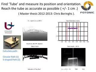
Find ‘Tube’ and measure its position and orientation.

Find ‘Tube’ and measure its position and orientation. Reach the tube as accurate as possible ( +/- 1 cm .)( Master thesis 2012-2013: Chris Beringhs ). Calculate path: Circular Path (1) S-shaped Path (2)

Precision navigation: Circular Path. RM = (xM²+zM²)1/2 x0 - xM= zM.tg(β) x0 . sin(ε)/x0 = sin(90°-β)/RM  sin(ε) . yA + L = RM.cos(ε) xA = RM.sin(ε) tg(γ) = (j-J2)/f (Image information). 1. Track correction over an angle (γ.sign(ε) +δ): |AP| = yP ( Circular path ! ) |AP|/sin(ε) = (yP+L)/sin(δ) [1] (Sine- yP/sin(ε) = RM/sin(ε+δ) [2] rule). From which: (yP+L)sin(|ε|) |sin(δ)| = ------------------------------------------------ (RM²-2.RM.(yP+L).cos(ε) + (yP+L)² )1/2 2. Drive with a radius Rx over an angle α: α = |ε| +|δ| , |Rx|= yP.tg(α/2)  ( AGV Radii LUT ) . So, yPmust be searched for …     Here: β, ε, γ < 0 ! M L x β ε Track (0,0) β Track Rx RM α γ P(xP,yP) δ x0 xM A( xA,yA) y

Precision navigation: Curcular Path(2) •    • 3. After track correction |AP| must equal yP ! • |AP|² = xA² + (yA-yP)² = yP² • xA² + yA² = 2.yA.yP • yP = (xA² + yA²)/2yA M x L ε Track P(xP,yP) zM Rx Track γ δ A( xA,yA) y

Precision navigation: S-shaped Path. RM = (xM²+zM²)1/2 x0 - xM= zM.tg(β) x0 . sin(ε)/x0 = sin(90°-β)/RM  sin(ε) . tg(γ) = (j-J2)/f (Image information). |ε| = |ε0| + |γ| m/sin(γ) = Z/ sin(ε) = RM/ sin(ε0) m² = Z² + RM² - 2.Z.RM.cos(γ) m = Z.sin(γ)/sin(ε) ; sin(ε0) = sin(ε).Z/RM m² = Z² + RM² - 2.Z.RM.cos(γ) Z = RM.sin(ε).sin(ε + γ) / [sin²(ε) – sin²(γ)] Angle α en radius Rk are bound by: Z.sin(ε0) + Rk.[1-cos(ε0)] cos(α + ε0 ) = 1 - ------------------------------ 2Rk d3 = Rk.sin(α + ε0 );  t3 = (α+ ε0)/ωk(Rk) d2 = d3 – Rk.sin(ε0);  t2 = α/ωk(Rk) m Here: β, ε, γ < 0 ! ε0 M L x β ε Z RM d3 β (0,0) d2 Rk γ -Rk α x0 δ xM A( xA,yA) y ε0 So, Rkmust be searched for …   LUT

ToF guided navigation of AGV’s. D2 = DP ? Instant Eigen Motion: translation. Random points P! (In contrast: ‘Stereo Vision’ must find edges, so texture is pre-assumed )

ToF guided navigation of AGV’s. D2 = DP ? Instant Eigen Motion: planar rotation. Image data: tg(β1) = u1/f ; tg(β2) = u2/f .Task: find the correspondence β1 β2 ; Procedure: With 0 < |α| < α0 With |x| < x0 xs = |x.sin(α)| ; xc = |x.cos(α)| . R = - x.cos(α)/[1-cos(α)] δ1 = |R.sin(α)| . Projection rules for a random point P : xP = D2.sin(β2) = D1.sin(α + β1) + xc zP = D2.cos(β2) = D1.cos(α + β1) + xs – δ1 D1.sin(α + β1) + xc tg(β2) = -------------------------------  u2 . D1.cos(α + β1) + xs – δ1 D2² = D1² + x² + δ1² + 2D1.x.sin(β1) - 2δ1.[D1.cos(α – β1) + xs] .  D2 . Next sensor position P z2 Here: x < 0 α < 0 R > 0 . D2 D1 DP z1 β2 β1 Previous sensor position α R+ δ1 x Parallel processing possible,Ransac driven !

ToF guided navigation of AGV’s. Instant Eigen Motion: planar rotation. e.g. Make use of 50 random points at the horizon. Ransac methods are advised. Ransac = RANdomSAmple Consensus . Result = Radius & Angle D2 = DP ? α R

VLAAMS INSTITUUT VOOR MOBILITEITWetenschapspark 13B-3590 DIEPENBEEK T +32 11 24 60 00 www.vim.be/projecten/sensovo Flemish Institute for Mobility: project ‘sensovo’. Make a choice of an adapted camera and its set up. (Benchmark the cameras). Data-captation: ~ 1 GByte / km. ( Width = 1.5 m / camera ) Identification of the road sections ( Section # + GPS start/stop + Image # + Speed ) Parallel computed image analysis: ‘edges’ on a level 2, 4 or 6 cm. (Prewitt filter + small contour closings if necessary). Transversal z-Plus/z-Min sequences. (e.g. track formation, convex road parts). Road cracks (e.g. concrete fractures, transversal and longitudinal stitches…). Contour interpretation and classification. Reports about the road damage on the level of kilometre, hectometre, decametre and meter. (List with the heaviest strokes on the scale of 1, 10, 100 en 1000 m ). Dealing with road paintings, mark signs (arrows..), ‘zebra strokes’...

Road inspections: MESA RS4500 (wide FoV). One trip = 200 km = 5 GB/1.5 m Width (speed independent). Camera: FOV ( 69° , 56 ° ) Resolution(176 , 144 pix); I = 172; J = 140 . Height z0 can be chosen (e.g z0 = 1.50 m): x0 = 2*z0*tg( 56° / 2) * (J-6)/J ; y0 = 2*z0*tg( 69° / 2) * (I-6)/I ; (overlap) Trigger period: T = 1000. y0 / v [msec] . Freq = v/y0 [ frames/sec ] = 5 Hz. Data generation: # images / km = 1000 / y0 (± 500 ).# doubles / image = 2 * 24000 = ± 50000# Mbytes / km = 200 / y0 (± 100 Mb/km ). v = 10 m/s = 36 km/h T = 10 msec (shutter). z0 = 1.50 m. y0 = 2.00 m.x0 = 1.50 m. About: ~ 15 x 15 mm² / pixel

Roadinspections: FOTONIC E-Series. One trip = 200 km = N * 16 GB/1.4 m (speed independent). Maximum fps = 60 !! Accuracy 0.01 m/m . v = 10 m/s = 36 km/h • One lateral stroke of 1.4 m. is multiple present in consecutive images. • Search for the damage in the centre of the images. • Steps: • Raw images should be deblurred • Row shifts are function of speed: • #i/I = v.T/y0  # i = floor(I*v*T/y0)Redundance Number N = floor(I/#i) T = 1.5 msec (shutter). z0 = 1.50 m. y0 = 2.00 m.x0 = 1.50 m. About: ~ 15 x 15 mm² / pixel

Averaging the distance to a fixed world point for a moving ToF camera: Z = Σk Z(uk,v)/K V = ds/dt 3.tk f u0 u-1 u-3 u3 u0 u1 k = [ -3 -2 -1 0 1 2 3 ] ; here: K = 7 . Disparity Law: (u0 – uk)/f = k.tk/zP , - (du/dt)/f = (ds/dt)/zP withtk = V.∆t [ mm ]. ∆t = 1/fps [ sec ] .vP = speed [pix/sec ] .vP/V = f/zP [ - ] . uk = u0 - k.(vP.∆t) uk = u0 - k.vimage , with: vimage [pix/image] u zP tk P

Data shuffling Reordering in such a way that road information present in different images can be averaged over dimension K . alternative modulation Melexis: EVK7530180x60 pix. M X Y A0 φ φ = f(X,Y) A2 A3 A4 A1 O km. 1 km. mlxGetDistances(rawFrameData,speed) At this moment ‘reordering’ is especially compatible with Melexis TOF cameras for which the data A1, A2, A3 and A4 are full available. A kind of saw teeth modulation is used in stead of a sine wave modulation. Collect the frames every 90°. If the speed is known (or measured) the pixel shift can be found and used in order to find associated mean-amplitudes from which the phase angles φ can be derived.

Motion deblur for ‘colour cameras ’ and for ‘ToF cameras’ ask for a different approach. • deblurring is structural incompatible with noise (cfr. Wiener Filters) ! • ‘pulsed ToF cameras’ react totally different from ‘phase shift ToF cameras’ ! • - the better we can handle ‘blur’ in real time the faster objects may flow ‘through’ the ToF-images. (VIM-project). Which pixels have ‘seen’ a specific dice eye and for what integration time. Let’s organize a ‘MARBLE experiment’ and benchmark different ToF camera types. (see next slide).

Marble experiments: a white ball rolling over a white floor ... , ( ...conveyor belts... ) coloured ball over (contrast) coloured floor. ToF Further research needed ! Point Spread Functions (PSF-depth / PSF-brightness) Question: … will white mice running in the snow give ToF - Motion Blur    ?

Spinning wheel experiments Materialedges Depthedges Use a bicycle wheel + a flat disk (PUR).Mount a pie shaped element (Thickness 40 mm , angle 30°).Mount a flat second material (Thickness 3 mm , angle 180°). Let it spin around and strange measurement phenomena will occur …

Moving ToF: (Robotics, AGV’s, conveyor belts,..‘road damage inspection’) During motion, inconsistent brightness values are collected giving rise to chaotic fluctuations on the measured phase angle ‘phi’ . Big deviations will occur ! φ = atan[(A1-A3)/(A2-A4)] Texture dependant mean intensity values 2.D = λmod . [φ/2π] 2 1 φ A1 A2 A3 A4 3 4 Remember: ‘pulsed time of flight cameras’ don’t follow this mechanism !

Spinning wheel experiment

Heavy noised brightness image

STATIC ~ 1000 mm ~ 1000 mm ~ 997 mm ~ 997 mm ~ 960 mm ~ 960 mm ~ 1000 mm ~ 1000 mm Z40 DYNAMIC ~ 997 mm ~ 1000 mm ~ 1000 mm ~ 960 mm

Distance image of a spinning wheel. Dark is closer, Bright is further away Z40. ~ 1000 mm ~ 997 mm ~ 960 mm ~ 1000 mm Distance ~ 1000 mm. Wheel diameter = 600 mm.

March 2013 Image Sensors ‘Motion blurreduced’ ToF-camerasbasedonpulsed ToF. www.TriDiCam.net Line sensor The firstline sensor with a resolution of 64 x 2 pixel to bedevelopedbyFraunhofer IMS. 15 kHz scan speed. www.odos-imaging.com Pixel shape Real.iZ 3 mm x 10000 Hz  30 m/s 108 km/u @ 10000 Hz  3 mm.

Frames per second: fps = 60 !! Strongly ReducedBlur Fotonic E70 E-Pan Jaguar (TexasInstr) Panasonic

Frames per second: fps = 60 !! ReducedBlur Fotonic Z70 E-Pan

Sheet of Light (SoL) Actual camera types can deal with 75.000 line acquisitions a second. The resolution depends on the FOV (e.g. FOV = 2000 mm.) and on the number of image columns (e.g. # cols = 2048). ∆x = # cols/FOV (e.g ∆x ~ 1 mm/pixel) ∆z = ∆x / sin(a) (e.g ∆z ~ 2 mm/pixel, a = 30° ) Row wise the sub pixel ‘Centre of Gravity CoG’ can be search for in 2k accuracy steps. In such case we get: ∆zCoG = ∆x / (2k.sin(a)) (e.g. ∆zCoG ~ 0.25 mm/pixel ) . v

ToF VISION: world to image, image to world - conversion RGBd- cameras P = [ tg(φ) tg(ψ) 1 d/D ] , P’ = [ tg(φ) tg(ψ) 1 ] . ( f is chosen to be the unit.) 1 j 1 J/2 i j0 J φ i0 ψ R horizon I/2 (0,0,f) A u.ku f = 1 D kr,kc r N v.kv d z I u = j–j0; uk = ku*u v = i – i0; vk = kv*v tg φ = uk/f tg ψ = vk/f r = √(xu²+f²) d = √(uk²+vk²+f²) D/d = x/uk = y/vk = z/f x y Every world point generates 12 important coordinates: x, y, z, Nx, Ny, Nz, N, kr, kc, R, G, B .

Pw c1 c2 z P1 P2 Cr1 f Cr2 c zr f N O1 xr c c yr b O2 STEREO VISION: ‘Disparity / Distance’ - Conversion • Image disparity [pixel]: • Set-up disparity [m]: • Object distance [m]: Error Estimation Rectified Images d = c2 - c1 f Stereo correspondence calculations are time consuming

Matlab programs ( Mesa / Fotonic ) ( easily extendable for Melexis, ODOS and other 3D-cameras) VR_fot_Wheel_Benchmark_zL / VR_Mesa_Wheel_Benchmark_DL VR_fot_Marble_Z / VR_MESA_Marble_Dzyx VR_EigenMotionRotation / VR_EigenMotionTranslation VR_Fot_Chris_ImageAnalysis / VR_Fot_Chris_AGV ( Image analysis & AGV-control ). OK_VR_Mesa_AcquireImageFast_DL_OoC

Find ‘Tube’ and measure its position and orientation.